Markets
Crypto, US stocks, and Nasdaq-100 — market cap and valuation data in one place.
US Stock Market Cap
The top ~1000 US-listed companies by market cap — live from Yahoo, categorized by sector. Choose a Top-N or a sector to view, click any stock to pull it into a selection pie, and compare against FMP.
| Ticker | Company | Price | Market Cap | P/E | P/B | P/S | TTM Revenue | Rev. Growth | FCF (Annual) | FCF (Qtr) | Div. Yield |
|---|
Nasdaq-100 Valuation Table
Sortable P/S, P/E, P/B, revenue growth, and free cash flow (annual + latest quarter) for the Nasdaq-100 — same data pipeline as the S&P 500 table (Robinhood + SEC EDGAR filings).
| Ticker | Company | Price | Market Cap | P/E | P/B | P/S | TTM Revenue | Rev. Growth | FCF (Annual) | FCF (Qtr) | Div. Yield |
|---|
Stock Research
Price chart with fundamentals, multi-LLM SEC filing analysis, and crowd sentiment — one ticker, one page.
📄 SEC Filing Analysis
🧭 Crowd Sentiment
📈 Price & Fundamentals
ETH Validators 💎
Live Ethereum beacon chain validator stats — active validators, queue sizes, total staked ETH, staking APR, and network participation rate. Data via beaconcha.in, refreshed every 60 seconds.
Vegas Weather 🌬️
Wind, gust, and sunrise/sunset for Las Vegas, NV — hardcoded for now, no location picker yet. Data via api.weather.gov + sunrise-sunset.org, refreshed every 5 minutes. No weather alerts shown.
Scores 🏈
Live scoreboard for the sports we track on Polymarket — college football to start, more to follow. Data via ESPN's public scoreboard API, auto-refreshed every 25 seconds while this tab is open.
Deuces Wild Bonus Poker
All 2s are wild. Edit the payoffs, pick your 5 dealt cards, hold what you want, then choose your draw cards.
Pay Table — payout at 5-coin max bet
Deck — click cards to choose 2 = wild
Solitaire
Klondike. Click a card to pick it up, then click where to move it. Double-click a card to send it to a foundation. Click the stock (top-left) to deal.
Polymarket 🔮
My filtered Polymarket — add the sports you care about and it shows the next game for each, winner only. Sign in with Phantom to trade. Auto-refreshes every 30s.
Premier League 2026-27 — Season Predictor ⚽
Drag the 20 clubs into your predicted final table, set your bonus picks, then save or share. Kick-off: 22 Aug 2026.
EFL Championship 2026-27 — Season Predictor 🏆
Drag the 24 clubs into your predicted final table. Top 2 go up automatically, 3rd–6th into the play-offs, bottom 3 down. Kick-off: Aug 2026.
EFL League One 2026-27 — Season Predictor 🥉
Drag the 24 clubs into your predicted final table. Top 2 go up automatically, 3rd–6th into the play-offs, bottom 4 down. Kick-off: Aug 2026.
EFL League Two 2026-27 — Season Predictor 🎖️
Drag the 24 clubs into your predicted final table. Top 3 go up automatically, 4th–7th into the play-offs, bottom 2 drop to the National League. Kick-off: Aug 2026.
English Football Power Rankings — Markov Chain 🔗
Ranks clubs by treating results as a Markov chain: each match sends a directed "importance" edge from loser to winner, weighted by goal margin (draws split both ways). Built from the last 3 years of results, linearly decayed to zero — this week's form counts fully, results from 3 years ago count for nothing. Each division also pulls in the one above/below so promoted and relegated clubs still rank.
Claude Code Usage 🤖
My live Claude Code subscription usage, read straight from this server's own logs — a public look at how much API-equivalent value a flat-rate plan delivers.
AI Market Map 🧠
A top-model comparison across the leading US and Chinese labs, plus the companies that power the AI industry grouped by the layer of the stack they play in — from foundation models down to the silicon. Search or filter by layer.
Security & Network 🛡️
Live server health — bandwidth, latency, connections, traffic, top IPs, and auto-flagged scanners. Refreshes every 5–10s.
Integrations 🔗
Manage third-party account connections. All tokens are stored server-side only and never sent to the browser.
Photos 📸
Browse your Google Photos library — albums, photos, and videos. Owner only.
Mail ✉️
Inbox for me@patd.dev — mainly account verification emails. Owner only.
🧠 The AI Debate
Working notes — building up from the very first artificial neuron toward modern models, one historical step at a time. Alongside the technical timeline, this page also tracks the major philosophical critiques of AI as they arise, and checks each one against how the field actually developed — some proved right, some wrong, some are still open.
1888 — Santiago Ramón y Cajal: The Neuron Doctrine
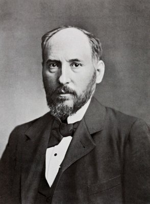
Before anyone could model "a neuron" as a discrete unit, someone had to prove neurons ARE discrete units.
Using Golgi's newly-invented staining technique, Cajal produced meticulous, detailed drawings showing the nervous system is made of separate, individual cells — neurons — with tiny gaps between them, not one continuous connected web as the rival "reticular theory" held. This became known as the neuron doctrine. Ironically, Cajal shared the 1906 Nobel Prize in Physiology or Medicine with Camillo Golgi himself, despite the two holding directly opposing views about how the nervous system worked.
This is the biological prerequisite for literally everything else on this page: McCulloch & Pitts' 1943 model (the very next relevant entry) treats a neuron as one discrete computational unit with its own inputs and output specifically because Cajal had already established, decades earlier, that this is biologically real — not a simplifying assumption, but an accurate reflection of actual nervous system structure.
1921 & 1953 — Ludwig Wittgenstein: Logic's Foundations, Then Its Own Best Critique philosophical throughline
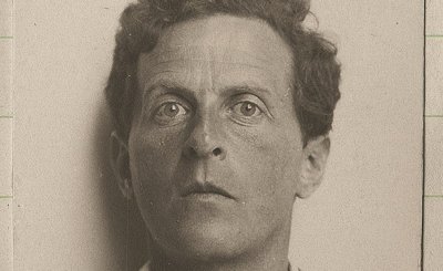
Predates AI as a field entirely — but supplied both its logical foundation and, decades later, its own deepest critique.
Wittgenstein appears twice in this story, arguing with himself across three decades. In 1921, his Tractatus
Logico-Philosophicus laid out the systematic truth-table method for propositional logic — proposition 5.101
gives the general formula for the number of possible truth-functions of n inputs, 2^(2^n), the exact
formula behind the "16 possible 2-input functions, 256 possible 3-input functions" discussion already covered on
this page. This is squarely in the tradition that later enables McCulloch-Pitts, Boolean logic gates, and formal
symbolic computation generally — the young Wittgenstein believed logic could exhaustively capture how language
pictures the world.
Then he spent his later career dismantling that picture. In the posthumously published Philosophical Investigations (1953), Wittgenstein rejected his own earlier framework — arguing that meaning doesn't come from fixed logical correspondence between language and world, but from use within social practices ("language games," "forms of life"). His "rule-following paradox" makes a very specific, sharp claim: no finite set of explicit rules can ever fully determine its own correct future application — any rule can be interpreted to fit multiple different continuations, so rule-following ultimately rests on shared practice and training, not on the rules themselves being self-interpreting. This is a direct philosophical ancestor of Dreyfus's critique below, decades before AI existed as a field to critique.
📄 Tractatus Logico-Philosophicus (1921), Project Gutenberg
1943 — Warren McCulloch & Walter Pitts
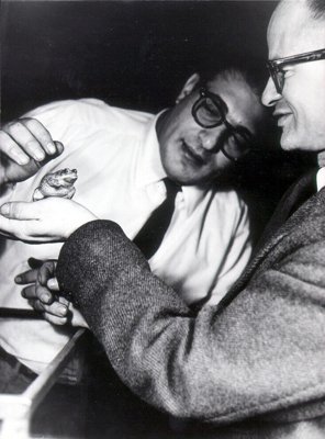
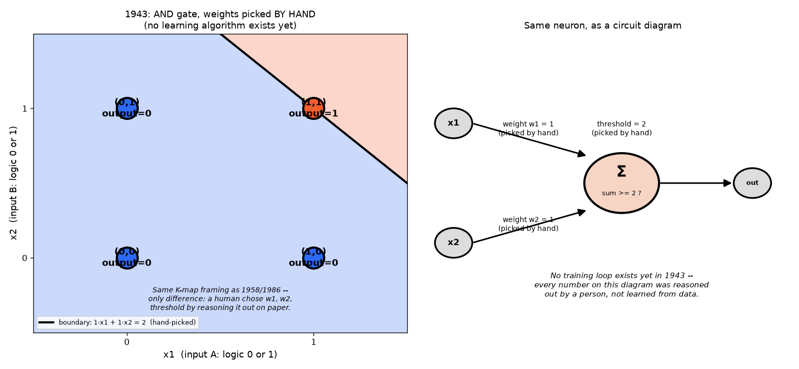
The first mathematical model of a neuron. Not trained — hand-designed.
McCulloch (a neurophysiologist) and Pitts (a self-taught logician) formalized what was already known experimentally about real neurons — Adrian's 1920s recordings had shown neurons fire in an all-or-nothing way, and there's a real, measurable voltage threshold that must be crossed before a spike fires. They turned this into pure math: multiply each input by a fixed, hand-chosen weight, sum them, and fire (output 1) only if the sum clears a threshold. No learning algorithm existed yet — the weights were picked by hand.
A single neuron built this way can compute AND, OR, and NOT just by choosing different weights/thresholds. It cannot compute XOR — no single straight-line boundary can separate that pattern, a limit that would matter enormously 26 years later.
Reading the diagram below, in EE terms: same Karnaugh-map-style plot and circuit diagram
as every later entry on this page — the only difference from 1958 onward is that here, a human reasoned out
w1=1, w2=1, threshold=2 on paper. There's no training loop yet to find these numbers automatically.
📄 A Logical Calculus of the Ideas Immanent in Nervous Activity (1943)
1949 — Donald Hebb: "Neurons That Fire Together, Wire Together"
The conceptual ancestor of every learning rule on this page — proposed before anyone had built a machine that could actually learn.
Hebb's book The Organization of Behavior proposed that learning happens through changes in synaptic strength: when one neuron repeatedly helps fire another, the connection between them gets stronger. His own summary, more precise than the popular one-liner: "when an axon of cell A... repeatedly or persistently takes part in firing [cell B], some growth process or metabolic change takes place... such that A's efficiency... is increased." Note this is purely correlational — cells that tend to activate together get a stronger connection — with no notion of a "correct answer" to compare against.
This is a genuinely different idea from Rosenblatt's 1958 perceptron rule (which arrives 9 years later): Hebb's rule strengthens connections based on co-activation alone, while the perceptron rule specifically corrects weights based on being wrong against a known target. Hebbian learning is the conceptual seed — a synapse's strength is not fixed, it changes with experience — that every error-driven learning rule on this page (perceptron, backprop) later sharpened into something usable for training toward a specific correct answer.
1950 — Alan Turing: "Computing Machinery and Intelligence"
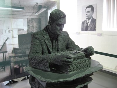
Not a neuron model at all — a completely different question: how would we even know if a machine could think?
Turing sidestepped the philosophically messy question "can machines think?" (he considered it too vague to be useful) and replaced it with something practical: the Imitation Game, now known as the Turing Test. If a human judge, holding a text conversation with both a person and a machine, cannot reliably tell which is which, the machine should be considered functionally intelligent — for practical purposes, regardless of what's "really" happening inside it.
This reframed the entire field around external behavior rather than internal experience — a genuinely different axis from McCulloch-Pitts' "how do you build a computing neuron," and one that's still argued about today (this is the same underlying question as the "stochastic parrots" debate about whether large language models "truly understand" anything, which we discussed earlier this session).
📄 Computing Machinery and Intelligence (1950), Mind
From Source Code to Hardware: a Real Compilation Pipeline
Turing is called the father of computer science for a reason — this whole pipeline is downstream of his theoretical work on what a "computer" fundamentally is and can do.
Turing's abstract "Turing machine" (from his earlier, even more foundational 1936 work, before the
Turing Test above) is the theoretical model underlying every real computer since — a precise definition
of what it means to "compute" something mechanically, step by step. Everything below is that abstraction
made concrete: all of this session's Python (and every neural network on this page) eventually becomes
real hardware instructions the same way any program does. Rather than describe that abstractly, here's an
actual simple adder function, compiled for real on this machine with gcc 13.3.0, showing
genuine output at every stage — not a fabricated example:
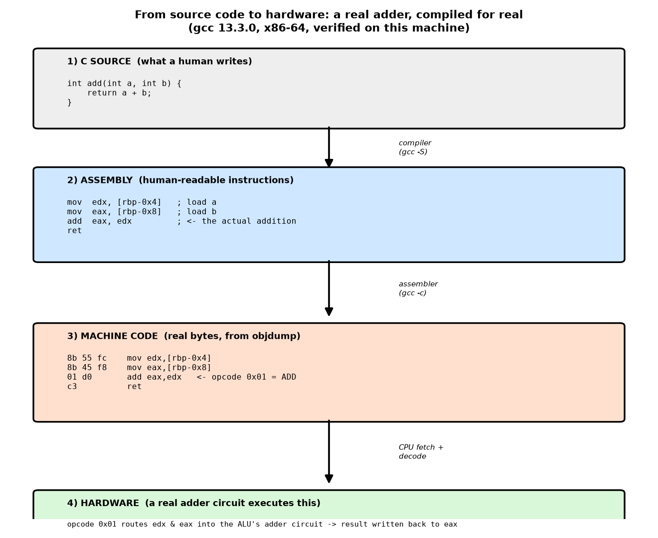
Reading the pipeline: the compiler turns C into human-readable assembly (stage 2) —
note the actual work is just one line, add eax, edx; everything else is just moving numbers
into and out of registers. The assembler then turns that into raw bytes (stage 3) — 01 d0 is
the literal machine code for that add instruction; 0x01 is x86-64's opcode for "add," and
d0 encodes which two registers to use. When the CPU fetches and decodes that byte, it
physically routes the two register values into the ALU's adder circuit — real transistors doing real
binary addition, the hardware endpoint of every abstraction on this page.
This is the same relationship as the McCulloch-Pitts neuron's sum ≥ threshold comparator
from the very first entry above: a mathematical operation described in software ultimately bottoms out as
a specific, physical arrangement of logic gates — whether that's a general-purpose CPU's ALU decoding an
opcode, or a dedicated neural-network ASIC with a hard-wired MAC (multiply-accumulate) unit built to do
nothing but that one operation, as fast as possible.
1952 — Hodgkin & Huxley: The Actual Circuit Model of a Neuron
Genuinely an EE-relevant entry — this is a literal circuit model (capacitor + variable resistors + batteries) of a real biological cell.
Using the (unusually large, easy to experiment on) squid giant axon, Hodgkin and Huxley worked out the actual ionic mechanism behind a neuron's electrical spike — the "action potential" already referenced back in the 1943 entry's mention of Adrian's 1920s all-or-nothing recordings, now given a precise, quantitative explanation. Their model represents the cell membrane as a capacitor, and each type of ion channel (sodium, potassium) as a variable resistor in series with a battery representing that ion's equilibrium voltage — four coupled differential equations describing exactly how these conductances change with voltage and time to produce a spike. This won them the 1963 Nobel Prize, and their equations are still the standard starting point for computational neuroscience today.
Where this fits on this page: McCulloch-Pitts' 1943 neuron reduces "does it fire" to a simple threshold comparison — accurate as a first approximation, but Hodgkin-Huxley is what that threshold actually looks like at the level of real ion channels opening and closing. Every artificial neuron on this page is a drastic simplification of this real circuit, trading biophysical accuracy for something trainable at scale.
The nonlinearity goes deeper than just the final spike, too. The Hodgkin-Huxley equations themselves are explicitly nonlinear — each ion channel's conductance depends on voltage through gating variables that follow their own nonlinear (sigmoid-shaped) curves, not a simple linear relationship. But real neurons are nonlinear in an even richer way than that single spike-or-not decision suggests: a neuron's dendrites (the branching input structure feeding into the cell body) aren't just passive wires summing up inputs linearly before reaching a single threshold — they contain their own voltage-gated channels, capable of local, nonlinear interactions within different branches of the same neuron, before any signal even reaches the main spike-generating threshold. Some real dendritic branches have been shown experimentally to compute something logically similar to AND or even XOR-like operations locally, using nonlinear dendritic interactions — meaning a single biological neuron may be capable of a small amount of the same "multiple comparator lines combined" computation that our artificial network needed two entire neurons to achieve back in the 1986 XOR entry. Every artificial neuron on this page — including the ones inside today's frontier transformers — collapses all of this rich, nonlinear, spatially-structured dendritic computation down to one linear weighted sum plus one simple nonlinear activation function. That's a real, deliberate loss of biological complexity in exchange for something trainable at massive scale, not evidence the artificial version is a faithful copy of the biological original.
1956 — The Dartmouth Conference
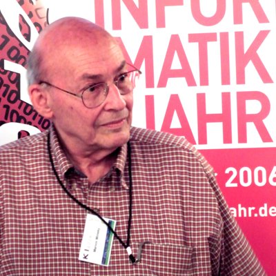
(1 of 4 organizers)
Where "Artificial Intelligence" was named as a field — no working system, just a founding event.
John McCarthy, Marvin Minsky (yes — the same Minsky from the 1969 critique below), Claude Shannon (the same Shannon whose 1937 thesis first showed Boolean logic could be built from relay circuits), and Nathaniel Rochester organized a summer workshop at Dartmouth College proposing that "every aspect of learning or any other feature of intelligence can in principle be so precisely described that a machine can be made to simulate it." That sentence is literally where the term "Artificial Intelligence" was coined.
No breakthrough system came out of the workshop itself — its real significance is that a scattered set of related ideas (cybernetics, information theory, automata theory, McCulloch-Pitts-style neuron models) got a single shared name and identity as one field for the first time, which is what let it start attracting dedicated funding and researchers.
📄 A Proposal for the Dartmouth Summer Research Project (1955)
1958 — Frank Rosenblatt's Perceptron
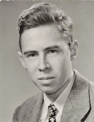
The real innovation: a neuron that changes its own weights from data.
McCulloch-Pitts neurons had to be hand-designed by a person who already knew the answer. Rosenblatt's breakthrough — built at Cornell, and physically realized as the Mark I Perceptron machine in 1960 (400 photocell "eyes" wired to adjustable resistors standing in for weights) — was a genuinely new idea: a simple rule for the neuron to correct itself, using only its own mistakes, with no human manually tuning anything.
The rule is almost embarrassingly simple: show it an example, let it guess, and if it's wrong, nudge every weight a little in the direction that would have made it right. Repeat.
Reading the diagram below, in EE terms: x1 and x2 are the two binary logic inputs (0 or 1)
feeding the neuron — think of them as two digital signal lines. The neuron computes a weighted sum
(a summing junction, like a summing op-amp: x1·w1 + x2·w2 + bias) and compares that sum
against zero, exactly like a comparator with its reference tied to ground: sum ≥ 0 → output HIGH (1),
sum < 0 → output LOW (0). The left plot is just a Karnaugh map for 2 inputs, but instead
of hand-circling groups of 1s, the boundary between regions is drawn by that comparator equation directly —
the black line is every point where the sum is exactly zero. The right diagram is the
exact same math, drawn the way a circuit/network diagram usually looks, with the real learned weight and
bias values labeled on each connection.
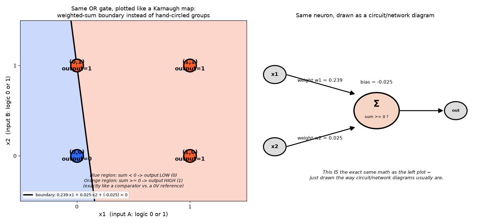
Where do 0.239 and 0.025 actually come from? This diagram now runs the real 1958 learning
rule to produce them — starting from small random weights, then repeatedly applying
new_weight = old_weight + learning_rate × error × input against the OR truth table until every
case is answered correctly. Notice the two weights aren't equal, and that's the honest, important part:
the perceptron rule only nudges a weight when its corresponding input was actually 1 for that example (the
rule multiplies by input, so a 0-input contributes no correction that round). Depending on the
random starting point and which examples happen to correct the weights first, training can validly land
on many different final lines that all correctly separate OR's four points — 0.239/0.025 here isn't "the"
answer, just one valid one this particular run converged to. Re-running with a different random seed would
converge to different (but equally correct) numbers.
This is the moment "training a model" — as opposed to "designing" one — was born. Every model we've run since (including the frontier ones) is a direct descendant of this same core idea: guess, measure the error, adjust the weights, repeat.
📄 The Perceptron: A Probabilistic Model (1958), Psychological Review
1959 — Arthur Samuel's Checkers Program parallel branch, not part of the neuron lineage
Coined the term "machine learning" — using a completely different technique from neurons.
Samuel, at IBM, built a program that played checkers against itself thousands of times, using a scoring function (an evaluation of how good a board position looks) combined with a search over possible future moves, and refined that scoring function based on which choices led to wins. Not a neuron, no weighted sum, no threshold — a different lineage entirely, based on game-tree search and self-play. It's the paper that literally coined the term "machine learning."
In a famous 1962 exhibition match it beat a strong human amateur player, generating major press coverage of "thinking machines" — a very public, concrete proof that a computer really could improve its own performance from experience, not just execute a fixed program.
1959–1962 — Hubel & Wiesel: The Visual Cortex's Hierarchy
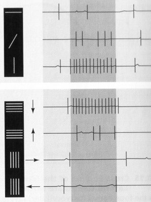
The direct biological inspiration for the CNN entry later on this page — this is not a loose analogy, it's a documented, named lineage.
Recording directly from neurons in a cat's visual cortex, Hubel and Wiesel discovered two distinct cell types: "simple cells" that respond strongly only to a specific, narrow orientation of edge (a vertical line, say) at one specific location, and "complex cells" that respond to the same kind of edge across a range of locations — achieving that flexibility, they proposed, by pooling input from many simple cells with the same orientation preference but different positions. This revealed the visual cortex as hierarchically organized: simple, local feature detectors feeding into progressively more complex, more position-tolerant ones. This won them the 1981 Nobel Prize.
This is a direct, documented inspiration, not just a loose parallel: Kunihiko Fukushima explicitly built his 1979/1980 Neocognitron — the direct architectural ancestor of the CNN entry later on this page — as a computational model of exactly this simple-cell/complex-cell hierarchy. The Neocognitron's local receptive fields and pooling layers are a direct translation of Hubel & Wiesel's biology into a trainable architecture, which LeCun's LeNet later refined with backpropagation.
1965 — Lotfi Zadeh's Fuzzy Logic parallel branch, not part of the neuron lineage
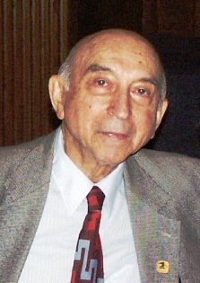
Truth as a matter of degree — but hand-designed, never learned from data.
Not a neural network technique at all, and not a step in the McCulloch-Pitts → Perceptron → backprop chain — a separate, contemporaneous idea. Zadeh's insight: real-world concepts like "warm" or "fast" don't have crisp boundaries, so instead of forcing truth to be strictly 0 or 1, let it be any value in between — 0.7 "true," representing a degree of membership rather than a hard yes/no.
A fuzzy system is built from human-written rules ("IF temperature is warm AND humidity is high THEN fan
speed is medium-high") using hand-designed membership functions — there's no training loop, no
loss.backward(), no learning from examples at all. It became a genuine commercial success
story in the late 1980s–90s, especially in Japan, showing up in washing machines, camera autofocus, subway
train controllers, and air conditioners — maturing at almost exactly the same moment neural networks were
just recovering from the AI winter via backpropagation.
Despite the "digital vs. analog" framing being tempting, fuzzy logic is almost always run as ordinary floating-point software on ordinary digital computers — it's a digital simulation of a continuous-valued idea, not literal analog hardware. (Ironically, it's modern neural networks' smooth activation functions that map most directly onto real analog computing chip research today.)
📄 Fuzzy Sets (1965), Information and Control
1969 — Minsky & Papert's Perceptrons
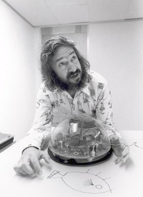
A rigorous proof of the single-neuron ceiling — and the start of the "AI winter."
Minsky and Papert mathematically proved what the 1943 model already hinted at: a single-layer perceptron can never solve XOR, or anything else that isn't linearly separable. They acknowledged that stacking multiple neurons into layers could in principle overcome this — but were openly pessimistic anyone would find a way to actually train such a stack. That pessimism, more than the limitation itself, is widely credited with gutting funding and interest in neural network research for over a decade.
1965–1972 — Hubert Dreyfus: "What Computers Can't Do" philosophical throughline
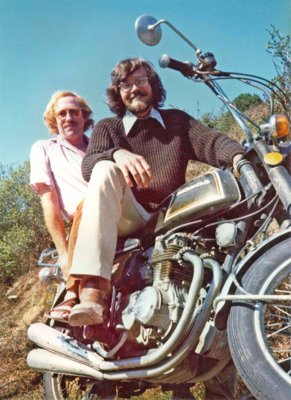
Berkeley philosopher's direct, sustained attack on symbolic AI — arriving years before the field itself recognized the problem.
Dreyfus's 1965 RAND paper "Alchemy and Artificial Intelligence" and 1972 book What Computers Can't Do (revised in 1992 as What Computers Still Can't Do) drew on Heidegger and Merleau-Ponty's phenomenology to attack the core assumption of "GOFAI" (Good Old-Fashioned AI) — that intelligence is fundamentally symbol manipulation according to explicit rules. His argument: human expertise is tacit, embodied, holistic, and contextual, not reducible to enumerable formal rules — genuine understanding requires being a body, situated in a physical and social world with real needs and stakes, not just processing symbols.
The AI community's reaction at the time was hostile, sometimes personally so. But his specific target — GOFAI — is exactly the Expert Systems paradigm in the very next entry below, and it collapsed for almost exactly the reasons he named: brittle, no genuine common sense, unable to handle context outside narrow hand-coded rules (what he and others called "the frame problem"). Notably, Dreyfus was not simply anti-AI — he held guarded optimism toward connectionist/neural-network approaches specifically because they're sub-symbolic and pattern-based, much closer to his own account of tacit understanding.
Late 1970s–80s — Expert Systems what "mainstream AI" actually was during the neural-network dark ages
A huge commercial boom, then a bust — and the real answer to "surely something happened in that gap."
While neural networks sat in the funding wilderness after Minsky & Papert, a completely different, non-neural approach dominated AI research and industry: expert systems — programs that encoded a human expert's knowledge as explicit IF-THEN rules, plus an "inference engine" that chained rules together to reach conclusions. MYCIN (Stanford, diagnosing bacterial infections) and XCON/R1 (Digital Equipment Corporation, configuring complex computer orders) were the famous examples — XCON reportedly saved DEC on the order of $40 million a year by the mid-1980s. This was a genuine, large-scale commercial AI boom, complete with dedicated LISP-machine hardware companies.
It collapsed starting around 1987 — hence "Expert Systems" being the actual majority of AI funding and attention during exactly the years neural networks were dormant. Every new rule had to be manually extracted from a human expert (slow, expensive "knowledge engineering"), the systems were completely brittle outside their narrow hand-coded domain, and the specialized LISP-machine companies got wiped out once cheaper general-purpose workstations became powerful enough. This collapse is specifically called the second AI winter.
1986 — Rumelhart, Hinton & Williams: Backpropagation
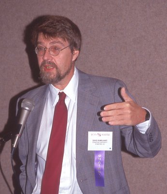
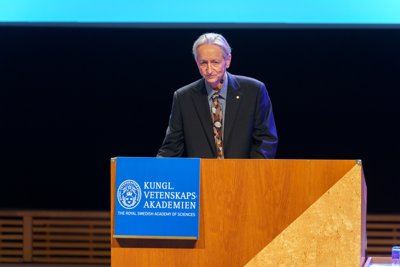
How to actually train a hidden layer — the fix that ended the winter.
The hard problem wasn't "use 2 neurons instead of 1" — it was figuring out how to assign credit/blame to a hidden-layer neuron's weights when you only know if the final output was right or wrong. This 1986 Nature paper demonstrated the fix: backpropagation, using calculus (the chain rule) to push the output error backward through every layer. It's the same algorithm — completely unchanged in its core math — behind every model we've trained on this site, including the tiny GPT-2 and the network below.
Here's a 2-hidden-neuron network, trained live via this exact algorithm, finally solving XOR:
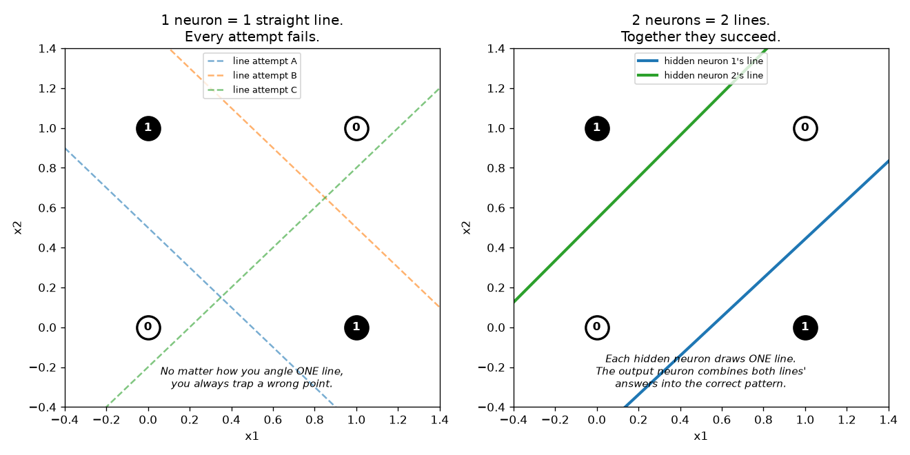
Any single straight line (left, dashed attempts) always traps a wrong point — mathematically impossible to avoid, since XOR's 1s and 0s sit on opposite diagonal corners. Two lines together (right) succeed.
Now the same network, drawn the EE way — two summing-junction/comparator neurons (h1, h2), each with its own real learned weights and boundary line, feeding a third comparator neuron that combines their two yes/no answers into the correct XOR result:
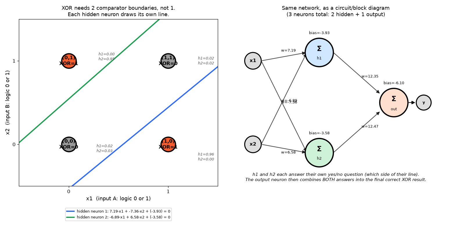
Each hidden neuron only ever answers one question — which side of its own line. Neither answer alone tells you XOR's correct output; only the output neuron's combination of both does. That combination step is exactly what a single neuron structurally cannot do.
📄 Learning representations by back-propagating errors (1986), Nature
1989 & 1998 — Yann LeCun: Convolutional Neural Networks (LeNet)
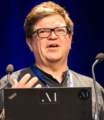
Same Yann LeCun who shows up later in this page's critiques section (2022, arguing pure LLMs are a dead end) — decades earlier, he was the one who made images practical for neural networks at all.
Every network on this page so far has been fully connected — every input wired to every neuron with its own independent weight (our XOR net, the perceptron). For an image, that's a real problem: a modest 200×200 pixel image has 40,000 inputs, and a fully-connected hidden layer would need a separate weight for every input-to-neuron connection — millions of weights before you've done anything useful, and no way to reuse what's learned about detecting an edge in one part of the image when that same edge shows up somewhere else.
LeCun's fix, applied practically in 1989 (reading handwritten ZIP codes for the US Postal Service at Bell Labs) and refined into the famous 7-layer LeNet-5 in 1998: a small filter — a tiny grid of shared weights, far smaller than the image itself — slides across the entire image, computing the same weighted sum at every position. The same 9 numbers detect a vertical edge whether it appears in the top-left corner or dead center — one filter, reused everywhere, instead of a separate weight for every pixel position. This is convolution, and it's the "C" in CNN.
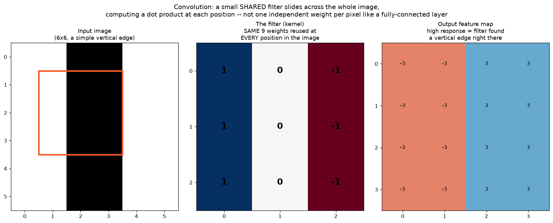
Stack several of these convolution layers (each followed by "pooling" — downsampling that keeps only the strongest response in each small region) and something powerful happens: early layers learn to detect simple local features like edges, exactly like the filter above; deeper layers combine those into progressively more complex shapes, textures, and eventually whole objects. LeNet-5 had about 60,000 parameters total — tiny by today's standards, but it's the direct architectural ancestor of the network in the very next entry.
1990 — Jeffrey Elman: The "Vanilla" Recurrent Neural Network
The first network on this page with a genuine memory — and the direct ancestor of the RNN/LSTM lineage.
Everything up to this point (perceptron, XOR net) has been feedforward: data goes in, flows straight through once, comes out — no memory of anything that came before. That's fine for a fixed input like two logic signals, but useless for a sequence (a sentence, read one word at a time), where what came earlier genuinely matters for what comes next.
The "recurrent" idea has an older, more tangled history than one clean date: the Hopfield Network (1982) was the first well-known network with feedback loops, though it's structured differently enough that it's not always counted as part of the same family; the Jordan Network (1986) first defined "recurrent" the way we mean it here (output feeding back into the hidden layer). Elman's 1990 network is the one usually meant by "plain RNN" today, and the first successfully trained with backpropagation.
The internal structure: at each time step, a single "cell" takes two things as input — the current word/token, and its own hidden state carried over from the previous step — and produces an output plus an updated hidden state that gets passed to the next step. That hidden state is the network's only memory of everything it's seen so far, compressed into one vector.
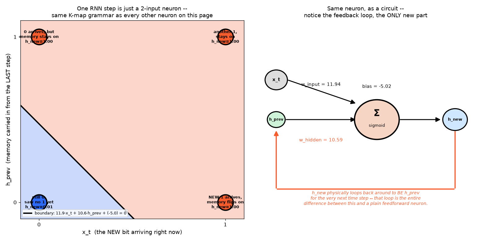
Reading this in the same K-map style as every neuron so far: at any single time step,
an RNN cell is just a 2-input neuron — its two inputs are the new incoming value (x_t)
and the memory carried in from the last step (h_prev), combined by a weighted sum + sigmoid,
exactly like the perceptron. The only genuinely new ingredient is the loop on the right: the output
(h_new) gets physically routed back around to become h_prev for the next step.
These are the real learned weights from actually training a minimal 1-hidden-unit RNN on a "remember if a
1 has ever appeared" task:
1997 — LSTMs: Solving Memory for Sequences
Backprop could now train hidden layers, but plain recurrent networks still "forgot" anything more than a few steps back.
Hochreiter & Schmidhuber's Long Short-Term Memory network addressed the specific problem the previous entry's ⚠️ box named: once you chain many small steps together (like reading a sentence word by word), the gradient signal from backprop tends to shrink to nothing (or explode) as it's pushed back through many steps — the "vanishing/exploding gradient" problem. LSTMs added explicit "gates" (learned mechanisms deciding what to keep, forget, or output at each step) that let a network carry information across many more steps reliably, without changing the basic recurrent shape from the entry above.
This became the dominant way to handle language, speech, and any sequential data for the next two decades — right up until the 2017 entry below replaced it.
Now zooming out to see many of these steps chained together over time, and how that compares to a Transformer processing the whole sequence at once instead:
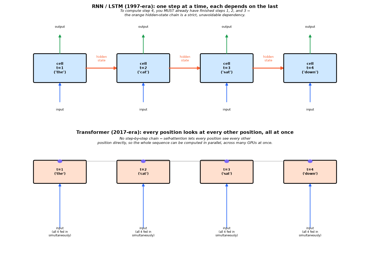
Look at the top half of the diagram: computing step 4 strictly requires steps 1, 2, and 3 to already be finished — that orange hidden-state chain cannot be skipped or reordered. This is exactly the "strictly sequential" limitation the ⚠️ box below describes, and it's the direct reason the 2017 entry replaced this architecture rather than just scaling it up further.
📄 Long Short-Term Memory (1997), Neural Computation
1999–ongoing — Ray Kurzweil: The Optimist's Case the counter-argument to everything above
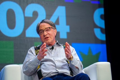
Every critique above assumes AI has real limits worth naming. Kurzweil's entire career is betting the limits are temporary.
Kurzweil's 1999 prediction — human-level AI (AGI) by 2029, and "the Singularity" (AI recursively self-improving beyond combined human intelligence, and merging with humans) by 2045 — long predates this entire LLM era, and he has not moved the date despite 25+ years passing, reaffirming 2029 in his 2024 book The Singularity Is Nearer. His argument rests on "the Law of Accelerating Returns" — information technologies improve exponentially, and exponential curves look deceptively flat right up until they don't.
His track record is genuinely contested, not simply good or bad: Kurzweil claims 86% accuracy on his own past predictions, and cites real, specific hits (smartphones, cloud computing, both predicted with real precision years in advance). But an independent 2019 assessment (Stuart Armstrong, Future of Humanity Institute) found only 42% accuracy — less than half his self-reported figure — largely because many predictions are vague enough to grade generously, or have timelines that quietly shift.
2012 — AlexNet and the ImageNet Moment
Backprop was 26 years old by now — what actually changed was data and compute, not the algorithm.
Alex Krizhevsky, Ilya Sutskever, and Geoffrey Hinton (yes — the same Hinton from the 1986 paper) trained a deep convolutional neural network on consumer GPUs and entered the ImageNet competition — 1000 object categories, 1+ million labeled training photos. It won by a shocking margin, roughly halving the error rate of the best non-neural-network approach in a single year. This is widely regarded as the moment that convinced the broader field deep neural networks, given enough data and compute, could dramatically outperform every hand-engineered alternative.
Why 2012, and not 1986? The algorithm hadn't changed — backpropagation is the same algorithm we ran ourselves. Two other ingredients finally caught up: enough labeled data existed (ImageNet itself, a massive human-labeled dataset assembled over the preceding years), and enough cheap, parallel compute existed — consumer GPUs, originally built for video game graphics, turned out to be extraordinarily well-suited to the matrix multiplications neural networks need. This is the exact "scaling" story from our earlier conversation this session, playing out for the first time.
📄 ImageNet Classification with Deep Convolutional Neural Networks (2012), NeurIPS
2014 — Ian Goodfellow: Generative Adversarial Networks (GANs)
Two networks locked in competition with each other — the dominant way to generate realistic images for the better part of a decade, before diffusion models took over.
Goodfellow's idea, reportedly worked out during a late-night discussion with friends in 2014: train two neural networks against each other in a zero-sum game. A generator network tries to produce fake images realistic enough to fool a second network; a discriminator network tries to correctly tell real images (from a training set) apart from the generator's fakes. Both networks improve together — as the discriminator gets better at spotting fakes, the generator is forced to get better at fooling it, and vice versa — a self-sustaining competitive loop rather than a single network learning from a fixed, direct target the way everything else on this page has so far.
2015 — Sohl-Dickstein et al.: Diffusion Models, the Theory
A genuinely different generative idea, borrowed directly from statistical physics — years before it was practical enough to matter.
"Deep Unsupervised Learning using Nonequilibrium Thermodynamics" proposed a different generative strategy entirely: instead of two networks competing (GANs), take real training images and gradually destroy them by mixing in more and more random noise, step by step, until nothing recognizable remains — this "forward process" needs no learning at all, it's just a fixed noising recipe. Then train a single neural network to do the reverse: given a noisier image, predict a slightly less noisy version of it. Chain that reverse step many times, starting from pure random noise, and — if it works — a realistic image gradually emerges.
This 2015 paper was purely theoretical grounding, explicitly inspired by non-equilibrium thermodynamics in physics — it did not yet produce results competitive with GANs, and the idea sat relatively unnoticed for five years until the next entry made it actually practical.
2017 — "Attention Is All You Need": The Transformer
Removed the strict step-by-step requirement entirely — the architecture behind every frontier model since, including the one you're talking to.
A team at Google introduced the Transformer, built around "self-attention" — instead of processing a sequence one step at a time carrying a hidden memory forward (the LSTM way), every position in the sequence looks directly at every other position simultaneously, weighing how relevant each one is to each other. This removed LSTMs' core bottleneck: since there's no step-by-step dependency, an entire sequence can be processed in parallel across many GPUs at once.
This is the exact architecture family behind the tiny GPT-2 we downloaded, trained, and ran earlier — and behind every current frontier model (GPT, Claude, Gemini, Llama). "Decoder-only causal transformer," the term from our very first conversation on this topic, refers to a specific way of using this 2017 architecture for next-token text generation.
Inside one block — this is the repeating unit that gets stacked N times (5 in our tiny demo, 96 in GPT-3, per the scale comparison above). Tokens get embedded into vectors, self-attention lets every position gather information from every other position at once, then a small feed-forward network (an ordinary MLP, the same building block from every network we've trained this session) processes each position — with "Add & Normalize" residual connections stabilizing training as this stacks very deep:
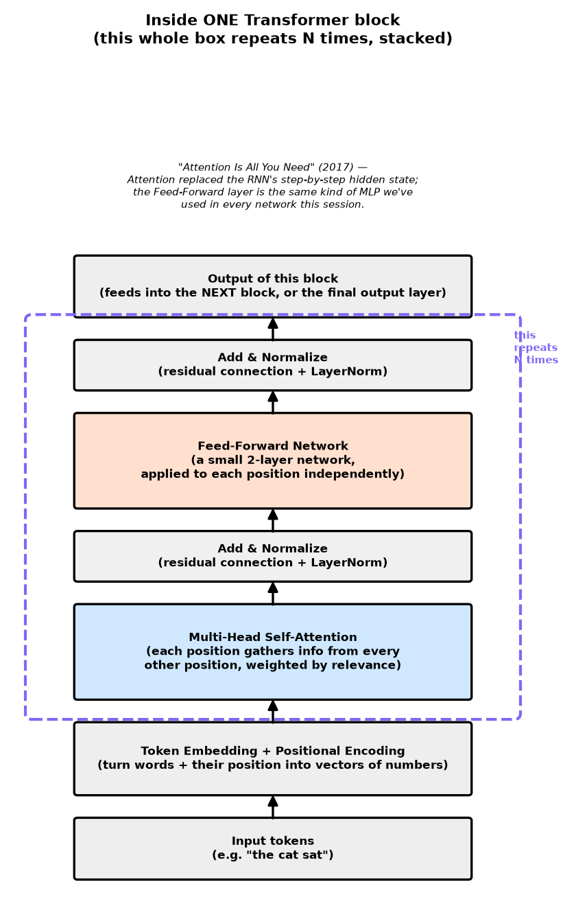
Forward propagation here is exactly the same concept as our XOR worked example above, just with far
more (and more complex) steps in between input and output — data flows up through this diagram, a real
number at every stage. Backward propagation is the same chain rule too, just automatically differentiating
through attention and the feed-forward layers instead of through two summing-junction neurons — the same
loss.backward() call, just walking back through a much longer chain.
📄 Attention Is All You Need (2017), arXiv
2018–ongoing — Gary Marcus: The Sustained Skeptic philosophical throughline
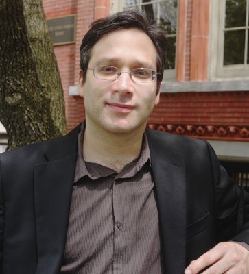
Cognitive scientist arguing, since before the current LLM boom, that pure deep learning needs to be paired with symbolic reasoning, not replace it.
Marcus's 2018 paper "Deep Learning: A Critical Appraisal" and 2019 book Rebooting AI (with Ernest Davis) predate ChatGPT by years, arguing that pure neural-network pattern-matching — no matter how large — would keep failing at tasks requiring genuine compositional reasoning, reliable factual grounding, and common sense, and that hybrid neuro-symbolic systems (combining learned pattern recognition with explicit symbolic reasoning) were necessary. He has remained a constant, high-visibility critic through the entire LLM era, frequently cataloguing specific failure cases (hallucinations, reasoning errors, brittleness on novel compositions) as evidence the underlying limitation hasn't actually gone away, just gotten harder to spot.
2018–2020 — GPT-1, GPT-2, GPT-3: The Scaling Era Begins
Same architecture as 2017, mostly just made bigger and bigger — and it kept working.
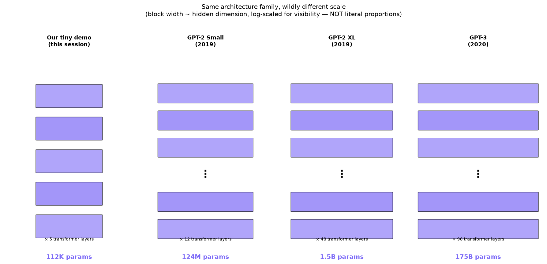
OpenAI applied the 2017 Transformer architecture specifically to the task of predicting the next word in huge amounts of text, at increasing scale: GPT-1 (2018, 117M parameters) proved the approach worked at all; GPT-2 (2019, up to 1.5B parameters — the same architecture as our tiny demo, just ~13,000x bigger) was notable enough that OpenAI initially withheld the full model over misuse concerns; GPT-3 (2020, 175B parameters) demonstrated "few-shot learning" — performing new tasks from just a handful of examples in the prompt, with no retraining at all.
Alongside GPT-3, OpenAI published empirical scaling laws (Kaplan et al., 2020) showing model performance improved smoothly and predictably as parameters, data, and compute all increased together — the empirical backbone of the entire "just make it bigger" era, and the same scaling-laws conversation we had earlier this session.
What "bigger" actually looks like — same architecture family throughout (the 2017 Transformer), just stacked deeper and wider each generation. Not drawn to scale or with every connection shown, just the shape (number of layers stacked) and the real parameter counts:
📄 Language Models are Few-Shot Learners (GPT-3, 2020), arXiv
2020 — Lewis et al.: Retrieval-Augmented Generation (RAG)
A direct answer to the "stochastic parrot"/hallucination problem — let the model look things up instead of relying purely on what's baked into its weights.
Lewis et al. (Facebook AI Research, University College London, and NYU), presented at NeurIPS 2020, proposed combining two different kinds of "memory": a language model's own parametric memory (whatever got baked into its weights during pretraining — everything covered in the entry above) with an external non-parametric memory — a real, searchable document collection the model can query at answer time. The mechanism has two parts: a retriever searches that document collection (typically using embedding-based similarity search) for passages relevant to the current question, and a generator (the language model itself) is given both the question and those retrieved passages as context, producing an answer actually grounded in real, specific source text rather than purely from statistical patterns memorized during training.
This directly addresses a concern from the Stochastic Parrots entry below: a model that can retrieve and cite real documents is at least partially checkable and groundable, rather than purely confabulating fluent-sounding text from training statistics. It also solves a separate, practical problem pretraining alone can't: giving a model access to information that's newer than its training cutoff, or specific to a private document collection, without needing to retrain the whole model.
2020 — Ho, Jain & Abbeel: DDPM Makes Diffusion Actually Work
The paper that turned 2015's theory into genuinely competitive image quality — the direct ancestor of every major image generator since.
"Denoising Diffusion Probabilistic Models" (UC Berkeley) refined Sohl-Dickstein's 2015 framework with specific, practical training choices that made the resulting image quality genuinely competitive with — and soon better than — GANs. Same core idea as 2015 (fixed forward noising, learned reverse denoising, illustrated below with our own tiny synthetic image), but with the specific mathematical and architectural refinements that made it actually work well in practice for the first time.
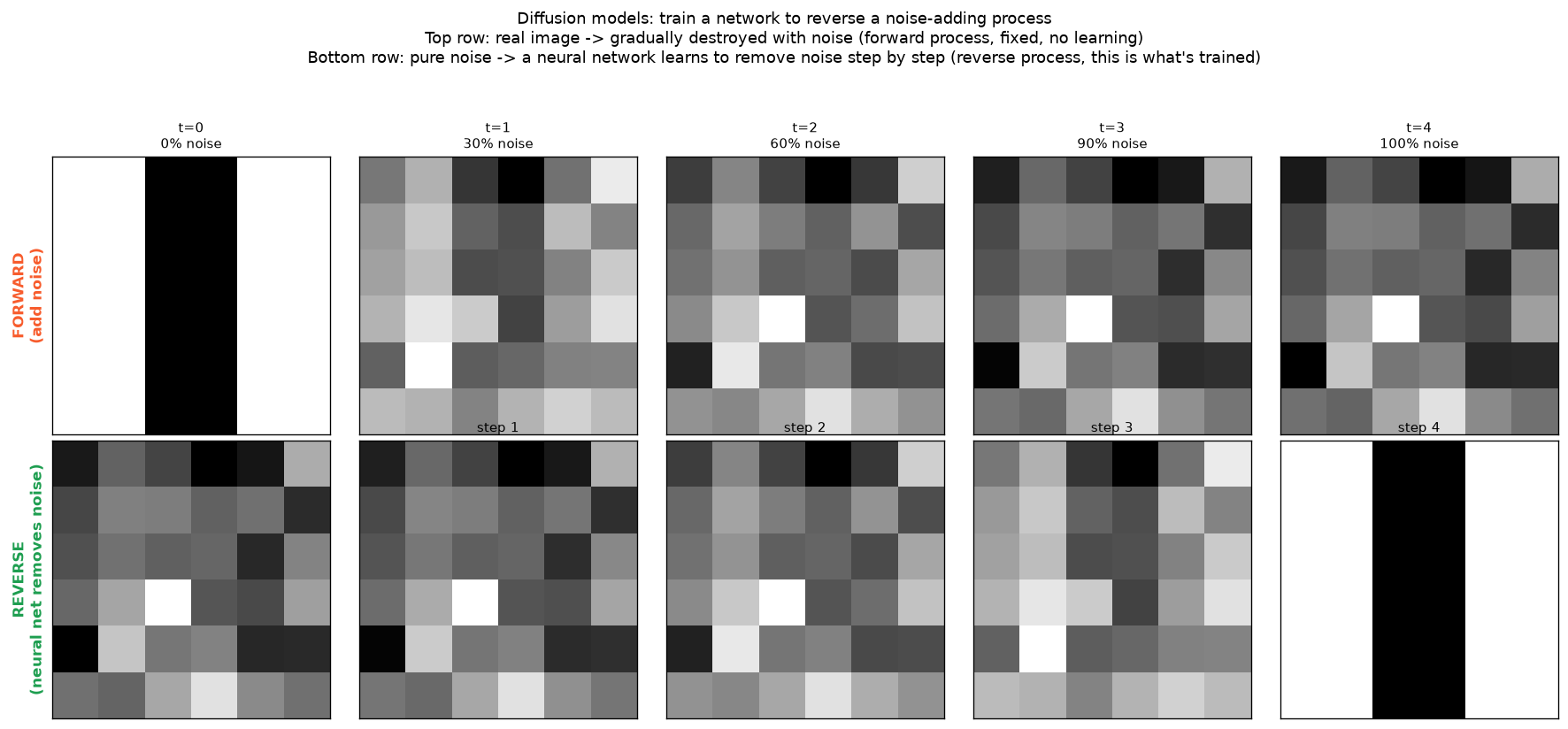
Honest note on the diagram above: the reverse row shown here just replays the same fixed noise sequence backward, to illustrate the concept clearly — a real trained diffusion model's reverse process is a genuinely learned neural network prediction at each step, not a simple replay, and actually training one from scratch is a much larger undertaking than the small demos elsewhere on this page.
2021 — "On the Dangers of Stochastic Parrots" philosophical throughline
The paper that coined the exact phrase used throughout this whole page's discussion of whether LLMs "understand" anything.
Bender, Timnit Gebru, and co-authors' 2021 paper argued large language models are sophisticated statistical pattern-matchers over text — "stochastic parrots" — fluently reproducing the form of language without any grounding in meaning, reference, or communicative intent. The paper's concerns went beyond philosophy: it raised the environmental cost of training ever-larger models, the risk of baking in and amplifying bias present in scraped training data, and the danger of fluent output creating an illusion of understanding that could mislead users and researchers alike.
This is the direct academic source of the "stochastic parrots" framing referenced repeatedly earlier in this same page's discussion of Dreyfus, embodiment, and whether frontier models "truly" understand anything — not just a casual phrase, but a specific, citable research position with real, ongoing influence on the field.
📄 On the Dangers of Stochastic Parrots (2021), ACM FAccT
2022 — DALL-E 2 & Stable Diffusion: Diffusion Goes Mainstream
The same year as ChatGPT's public moment (next entry) — 2022 was when generative AI broadly, not just text, reached the public all at once.
OpenAI's DALL-E 2 (April 2022) combined a diffusion model with CLIP (a separate model trained to understand the relationship between images and text captions), letting a written prompt guide the reverse denoising process toward an image matching that description — the key ingredient that makes "type a sentence, get a picture" possible at all. Stable Diffusion (Stability AI, LMU Munich, and RunwayML, August 2022) used the same underlying diffusion approach but was released publicly and openly — the model weights themselves, not just an API — making high-quality text-to-image generation runnable on a consumer GPU for the first time, a genuinely different accessibility choice from DALL-E 2's closed, hosted-only approach.
2022 — ChatGPT: The Public Moment
Not a new architecture — a product/interface moment that made this whole lineage visible to the world.
ChatGPT wrapped an already-existing GPT-3-family model in a simple chat interface and made it free and public. Nothing about the underlying 2017-architecture technology was new — what changed was accessibility. It became one of the fastest-adopted consumer products in history, and is the moment "AI" (specifically, this decoder-only-transformer lineage) went from a research/enterprise topic to mainstream public awareness — directly setting the stage for the investment, hype, and scrutiny (including the DeepSeek distillation disputes) we discussed earlier this session.
2022–ongoing — Yann LeCun: "Autoregressive LLMs Are a Dead End" philosophical throughline, still unresolved
A living, current critique from deep inside the field itself, not yet a settled historical verdict like Dreyfus.
LeCun (Turing Award winner, former Meta Chief AI Scientist) has argued publicly since 2022 that autoregressive LLMs — predicting one token at a time, exactly the mechanism behind our own tiny GPT-2 and every model in the 2018–2020 entry above — are fundamentally limited: small errors compound token by token, and the architecture has no genuine model of the physical world, so it "can't truly reason or plan" or predict the consequences of actions. His alternative, JEPA (Joint Embedding Predictive Architecture), predicts outcomes in a compressed, abstract representation space instead of generating output token by token — closer, in his view, to how a brain runs a fast mental simulation rather than imagining every physical detail.
Unlike Dreyfus, this critique is unresolved in real time — LeCun has continued pursuing this direction independently, and whether JEPA-style world models overtake pure autoregressive scaling, get absorbed as one component of hybrid systems, or turn out to be unnecessary is a genuinely open question this page cannot yet give a historical verdict on.
2023 — Noam Chomsky: "The False Promise of ChatGPT" philosophical throughline
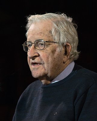
A linguistic critique, distinct from Dreyfus's phenomenology or LeCun's world-models argument.
Chomsky and co-authors' 2023 New York Times op-ed argued LLMs are categorically different from, and inferior to, genuine human language ability. His decades of linguistic theory hold that human language reflects an innate, universal grammar — a genuine generative system capable of understanding deep structure, causation, and what is impossible as well as what's likely. LLMs, by contrast, are statistical engines fitting patterns in existing text — capable of describing what usually happens, not explaining why, and just as able to learn "possible" and "impossible" human languages equally well, which he takes as proof they aren't modeling anything like real linguistic competence at all.
2024–2025 — Reasoning Models & Test-Time Compute (o1/o3)
The second scaling axis — already discussed this session, formally added here now.
As pure pretraining scale (bigger models, more data) started showing diminishing returns, OpenAI's o1 (and successor o3) introduced a different lever: instead of answering immediately, the model generates an extended internal chain of reasoning steps before producing a final answer, using reinforcement learning during training to learn to reason well, then spending more compute per question at the moment you actually ask it something — "thinking longer" on harder problems.
2024 — Anthropic: The Model Context Protocol (MCP)
Not a model or a training technique — a standardized plug for connecting AI to tools and data, and literally what's running underneath this very conversation.
Anthropic open-sourced MCP on November 25, 2024: an open standard for how an AI assistant connects to external tools, data sources, and services — Google Drive, GitHub, a database, a trading platform, anything — without every single AI application needing its own bespoke, one-off integration code for every tool it wants to use. An "MCP server" wraps access to one specific tool or data source in a consistent, discoverable format; any MCP-compatible AI client (like Claude Code, running this session) can then connect to any MCP server and use its capabilities the same standardized way.
This is directly, concretely running right now, not an abstract example: the EDGAR filings lookup, the Robinhood trading tools, and the sentiment-analysis tools available in this very environment are real MCP servers — and everything on this page was built by an MCP client (this conversation) calling them.
Adoption was unusually fast and unusually cross-company for a standard originated by one AI lab: OpenAI adopted MCP across its own products by March 2025, Google DeepMind added support in Gemini by April 2025, and Microsoft/GitHub joined its steering committee by May 2025. In December 2025, Anthropic donated MCP to the Agentic AI Foundation, a Linux Foundation project co-founded with Block and OpenAI — turning a single-company standard into genuinely neutral, shared infrastructure.
Full text timeline now complete through today — next pass: go back through and discuss/fix each entry in depth, plus add per-entry diagrams where useful.
👥 Who's Building This: Key Researchers Today
Not a ranking — a working roster of the people whose names show up most across current frontier AI, and what they specifically contributed.
The Transformer authors — Google Brain, 2017
Worth stating plainly: the architecture behind every current frontier model, including the one you're talking to, came out of Google — not OpenAI, not DeepMind.
Vaswani, Shazeer, and five co-authors (Jakob Uszkoreit, Illia Polosukhin, Aidan Gomez, Łukasz Kaiser, Niki Parmar) wrote "Attention Is All You Need" at Google Brain in 2017 — already the subject of its own entry earlier on this page. Shazeer specifically later left to co-found Character.AI, then returned to Google in 2024 — a good example of how fluidly researchers move between these companies.
Dario Amodei — Anthropic

Co-authored the actual scaling-laws paper already referenced in the 2018–2020 GPT entry above, before founding the company that builds the model answering these questions right now.
Amodei was a co-author on GPT-2 and GPT-3 at OpenAI, and on the Kaplan et al. scaling-laws paper — the empirical backbone of the "just make it bigger" era already covered on this page. He left OpenAI in 2021 to found Anthropic, with a safety-focused research agenda as the founding motivation.
Demis Hassabis — Google DeepMind
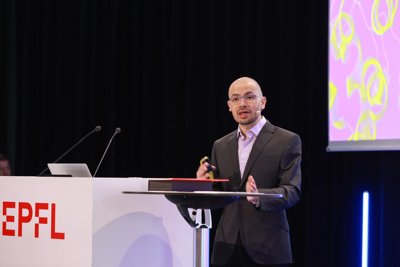
Co-founded DeepMind, acquired by Google in 2014 — now "Google DeepMind."
Led AlphaGo (2016, beat the world Go champion using reinforcement learning + tree search, a genuinely different technique family from anything on this page's neural-network timeline) and AlphaFold (protein structure prediction) — the latter won him the 2024 Nobel Prize in Chemistry, awarded the same year Hinton won the Physics prize for backpropagation-adjacent work.
Fei-Fei Li — Stanford
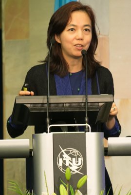
Built the dataset, not the model — but without it, the 2012 AlexNet entry on this page doesn't happen.
Li led the creation of ImageNet — the massive, human-labeled image dataset (1000 categories, 1M+ images) that AlexNet was trained and evaluated on. A direct, concrete reminder that the "scaling" story on this page isn't just about bigger models — it needed bigger, well-labeled datasets just as much.
Andrej Karpathy — educator and practitioner
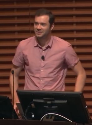
Former Tesla Autopilot lead and OpenAI founding member, now best known for making exactly this kind of from-scratch, verified, no-magic teaching material.
His minGPT/nanoGPT projects — small, fully transparent, from-scratch GPT implementations anyone can read top to bottom — are close in spirit to this whole page's own approach: build the tiny real version yourself rather than take the architecture on faith.
Jeff Dean — Google Chief Scientist
Built the infrastructure the rest of this section runs on, more than any specific model.
Co-created TensorFlow and led Google's large-scale distributed training systems — the software plumbing that makes training models at the scale described in this page's "model scale comparison" section physically possible in practice, not just on paper.
Already covered elsewhere on this page
Geoffrey Hinton, Ilya Sutskever, and Yann LeCun all appear in full earlier — Hinton and Sutskever in the 1986 Backprop and 2012 AlexNet entries, LeCun in the critiques section above (2022–ongoing, JEPA/world models) — rather than repeating them here.
🔬 Concept Deep-Dives
Not part of the chronological timeline above — standalone explainers for specific mechanics that come up repeatedly.
📋 Cheat Sheet / Glossary
Every term used across this page, in one place — vocabulary accumulates fast over a multi-day project.
Building Blocks
- Neuron
- The basic unit: multiply each input by a weight, sum them plus a bias, then pass the result through an activation function.
- Weight
- A number multiplying one input — how much that input matters to this neuron. Learned from data (1958 onward), not hand-picked (1943).
- Bias
- A constant added to the weighted sum, independent of any input — shifts the decision boundary off the origin. See the 1958 entry for why this matters.
- Activation function
- What turns the weighted sum into the neuron's output — step (hard on/off), sigmoid, ReLU, or GELU. See the Activation Functions deep-dive.
- Threshold / comparator
- EE framing of activation: a neuron firing at
sum ≥ 0is exactly a comparator firing at a reference voltage.
Architectures
- Perceptron
- Rosenblatt's 1958 single trainable neuron. One neuron, no hidden layer — a "network" of size one.
- Hidden layer
- Any layer of neurons between input and output. "Hidden" means not part of the input/output interface — not unobservable; we can and do inspect it directly.
- Multi-Layer Perceptron (MLP) / feedforward network
- Neurons arranged in layers, data flows straight through once (no loops). Our XOR network is the simplest real example.
- Feedforward
- Data moves one direction only, input toward output, no feedback loops — as opposed to recurrent.
- RNN (Recurrent Neural Network)
- Processes a sequence one step at a time, feeding its own previous output/hidden-state back in as memory. Not the same word as "Recursive" Neural Network (a different, rarer, tree-structured architecture). We have not built an RNN this session — only diagrammed one for comparison.
- LSTM (Long Short-Term Memory)
- A specific gated RNN design (Hochreiter & Schmidhuber, 1997) that fixes plain RNNs' vanishing-gradient problem over long sequences.
- Transformer
- The 2017 architecture ("Attention Is All You Need") behind every current frontier model. Processes all sequence positions in parallel via self-attention, instead of RNN's one-step-at-a-time approach.
- Self-attention
- The mechanism inside a Transformer where every position looks at every other position at once, weighing relevance, instead of relying on a passed-along hidden state.
Training
- Supervised learning
- Training data includes the correct answer for every example (what all our demos this session have used). Unsupervised = no correct answers given, algorithm finds structure on its own.
- Loss function
- A number measuring how wrong the current output is versus the correct answer — what training tries to minimize.
- Gradient descent
- Adjusting parameters in the direction that reduces the loss, using the loss function's derivative (gradient).
- Backpropagation ("backprop")
- The 1986 algorithm for computing that gradient for every weight in a multi-layer network, via the chain rule, working backward from the output.
- Chain rule
- The calculus rule that lets you multiply local derivatives together across layers to get a gradient for an early weight — see the worked XOR example above.
- Learning rate
- How big a step each weight update takes. Too small = slow; too large = coarse/unstable (in gradient-descent methods — the plain perceptron rule is more forgiving, per the Perceptron Convergence Theorem).
- Epoch
- One full pass through the entire training dataset.
- Linearly separable
- A problem solvable by a single straight-line (or hyperplane) boundary. AND/OR are; XOR/XNOR are not — the core reason multi-layer networks are needed at all.
Scale & Modern Practice
- Parameters
- The total count of learned weights + biases in a model. Our tiny demo: 112K. GPT-3: 175B.
- Scaling laws
- Empirical finding (Kaplan et al., 2020) that performance improves smoothly and predictably as parameters/data/compute all grow together.
- Fine-tuning / SFT (supervised fine-tuning)
- Further training an already-pretrained model on human-written example responses, to align its behavior.
- RLHF
- Reinforcement Learning from Human Feedback — trains a separate reward model on human preferences, then uses RL (typically PPO) to optimize the model against it. See the "RLHF and DPO" deep-dive below for the full pipeline.
- DPO
- Direct Preference Optimization — mathematically collapses RLHF's two stages (reward model + RL) into one direct optimization on preference data, no separate reward model or RL loop needed.
- Reasoning models / test-time compute
- o1/o3-style models (2024–2025) that spend extra compute "thinking" via an internal chain of steps before answering, rather than answering instantly.
Software / Hardware Pipeline
- Compiler
- Translates source code into assembly (and eventually machine code). Heuristic-based, not perfect — see the gcc
-O0vs-O2comparison. - Assembly
- Human-readable mnemonics for CPU instructions, one step above raw machine code bytes.
- Machine code
- The actual bytes the CPU executes — e.g.
01 d0for our adder'sadd eax, edx. - Object file (
.o) - Compiled machine code plus a manifest of what it defines/needs — not yet a runnable program.
- Linker
- Combines object files, resolving each undefined symbol to a real final address, producing one runnable executable.
- Interpreted language
- Executed by another program (an interpreter) reading it step-by-step at runtime, rather than compiled fully to native machine code ahead of time. Python via CPython is interpreted; C is compiled.
- JIT (Just-In-Time compilation)
- Compiling hot code paths to real machine code at runtime, after observing they're actually used a lot — see the Numba demo.
Architecture Shapes, Side by Side
Feedforward, Recurrent, Transformer, Recursive, CNN, GAN, Diffusion — same basic ingredient (neurons + weights), seven very different connection patterns.
Not to scale, and not every connection drawn — just the structural shape of how data flows through each one:
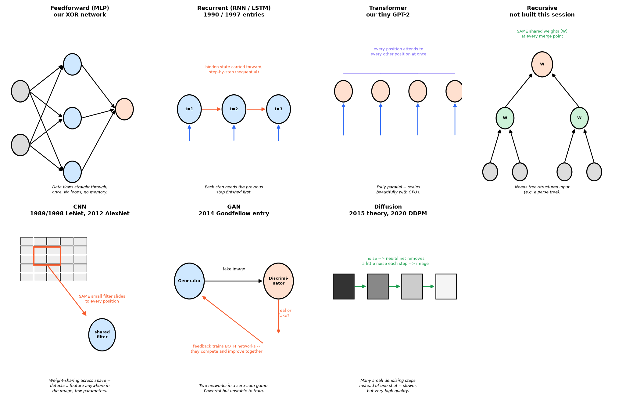
| Architecture | Data flow | Good at | Bad at | Real examples |
|---|---|---|---|---|
| Feedforward (MLP) | Straight through, once. No loops, no memory of previous inputs. | Fixed-size inputs with no inherent order/sequence — tabular data, simple classification. Fast, simple, easy to train. | Anything with sequence or variable length (text, audio, time series) — has no way to use position/order information at all. | Our XOR/OR-gate networks; the feed-forward sub-layer inside every Transformer block. |
| Recurrent (RNN / LSTM) | One step at a time, carrying a hidden-state "memory" forward — each step depends on the last. | Sequences where order matters and length varies — was the standard for language/speech/time series for ~20 years. | Strictly sequential — cannot parallelize across a sequence, so training on huge datasets is slow. Long sequences still lose earlier context even with LSTM's fixes. | Pre-2017 machine translation, speech recognition, older predictive-text keyboards. |
| Transformer | Every position attends to every other position simultaneously — fully parallel, no step-by-step dependency. | Sequences at massive scale — parallelizes perfectly across many GPUs, captures long-range relationships directly. | Attention cost grows quadratically with sequence length — very long inputs get expensive. Needs lots of data/compute to train well from scratch. | GPT, Claude, Gemini, Llama — every current frontier language model, plus our own tiny GPT-2 demo. |
| Recursive | The same shared weights applied repeatedly, merging pairs of nodes upward through a tree structure to one root. | Data that's naturally tree-shaped — parsing sentence grammar structure, some program-analysis tasks. | Needs the tree structure to already be known/given — doesn't generalize to plain sequences or unstructured data, so it's a niche choice today. | Historical NLP sentiment/parsing research (e.g. Stanford's Recursive Neural Tensor Network) — largely superseded by Transformers now. |
| CNN | A small filter of shared weights slides across the whole input, computing the same operation at every position — not one independent weight per input like a fully-connected layer. | Grid-structured data, especially images — detects a learned feature (an edge, a texture) anywhere it appears, with far fewer parameters than a fully-connected layer would need. | Data with no natural grid/spatial structure — the weight-sharing assumption that makes CNNs efficient for images doesn't help (or apply) for arbitrary tabular or sequence data. | LeNet-5 (1998), AlexNet (2012), most image classifiers; also the feature-extraction backbone inside many diffusion models below. |
| GAN | Two networks in competition: a generator produces fake examples, a discriminator tries to tell real from fake — both improve by trying to beat each other. | Generating sharp, realistic samples quickly — a single forward pass through the generator produces a full image. | Notoriously unstable to train — the two networks can fail to converge together, or the generator can collapse to producing only a narrow range of outputs ("mode collapse"). | Deepfakes, early realistic face generation (StyleGAN), largely displaced by diffusion models for image generation since ~2021. |
| Diffusion | A fixed process gradually adds noise to real data until it's pure static; a neural network is trained to reverse that, removing a little noise at a time across many steps. | High-quality, diverse image (and increasingly video/audio) generation — currently the dominant approach for text-to-image and text-to-video systems. | Slow to generate from — producing one output means running the reverse denoising step many times in sequence, historically much slower than a GAN's single pass (active research area). | DALL-E 2, Stable Diffusion, Midjourney, Sora-style video generation. |
How Alignment Training Actually Works: RLHF and DPO
The step that turns a raw next-word predictor into something that behaves like an assistant — separate from, and after, the pretraining covered in the GPT-era entries above.
A freshly pretrained model (next-token prediction on huge amounts of raw text, fully self-supervised — no human labels involved) has no built-in notion of "helpful," "harmless," or "follow the instruction I actually gave you." Getting from that raw predictor to something that behaves like an assistant takes a further training stage, and there are two different ways the field does it.
RLHF (Reinforcement Learning from Human Feedback) — the original approach, five steps:
1) Start from the pretrained model. 2) Optionally fine-tune it on human-written example responses first (ordinary supervised learning — "supervised fine-tuning," SFT). 3) Instead of paying humans to write full answers (expensive), show them several different model-generated responses to the same prompt and just ask which one is better — ranking is far cheaper than writing. 4) Use that preference data to train a separate reward model — a second neural network whose only job is predicting how a human would rate any given response. 5) Run reinforcement learning (typically an algorithm called PPO) on the original model: generate a response, have the reward model score it, nudge the weights toward whatever scores higher — repeated many times, with no human needed in the loop for each individual step, since the reward model stands in for one.
The honest limitation with RLHF: the reward model is only an approximation of real human preference, and the reinforcement-learning stage can learn to exploit that approximation's blind spots rather than genuinely improve — sounding confident and polished without actually being better. This is called reward hacking, a real, known, unresolved tension in the technique.
DPO (Direct Preference Optimization, Rafailov et al., 2023) — the same goal, one stage instead of two: DPO's actual contribution is a mathematical one — it proves the entire RLHF objective can be solved directly, without ever training a separate reward model or running reinforcement learning at all. Given the same preference data (human picks response A over response B), DPO trains the model directly to raise the probability of the preferred response and lower the probability of the rejected one, using a closed-form loss derived from the same underlying preference math RLHF's reward model was already built on — essentially treating "which one did the human prefer" as a direct classification problem, not something you need an intermediate reward-scoring model and a full RL loop to approach.
What that buys you in practice: no separate reward model to train and maintain, no RL sampling loop, no PPO stability issues to tune around, and less exposure to reward hacking — since there's no separate reward-model proxy sitting in between the preference data and the final model for the optimization to over-fit against.
Activation Functions: Step → Sigmoid → ReLU → GELU
The EE analogy: not a perfect switch, but a transistor's real, soft I-V transition region.
The 1943 neuron used a step function — a hard, instant jump from 0 to 1 at the threshold, exactly like an idealized digital switch. But a real transistor doesn't switch perfectly instantly either — it has a soft "knee," a transition region where it's neither fully off nor fully on. Sigmoid, ReLU, and GELU are different mathematical ways of building that soft transition on purpose.
Sigmoid (which you already know): 1 / (1 + e^-x) — a smooth S-curve,
output always strictly between 0 and 1, approaching but never quite reaching either extreme.
GELU (Gaussian Error Linear Unit — what our tiny GPT-2's config called "gelu_new"):
GELU(x) = x · Φ(x), where Φ(x) is the standard normal (Gaussian) cumulative
distribution function — literally "the probability that a standard normal random variable is less than x."
Intuitively: for a large positive input, Φ(x) ≈ 1, so GELU(x) ≈ x (passes through almost unchanged). For a
large negative input, Φ(x) ≈ 0, so GELU(x) ≈ 0 (mostly zeroed out). Near zero it's smooth and — notably —
dips slightly below zero for small negative inputs, unlike ReLU which clips negatives to exactly 0.
The specific "gelu_new" variant uses a faster tanh-based approximation of Φ(x) rather than computing the
exact Gaussian integral, since tanh is cheaper to compute at the scale of billions of calls.
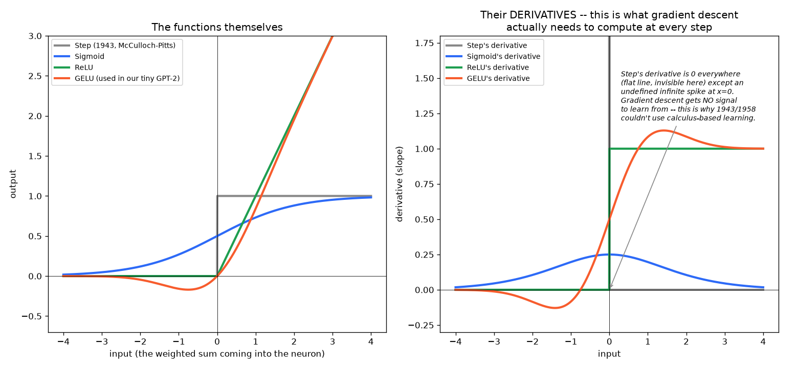
The right panel — the derivatives — is the important one, and it's the direct answer to the next question below: gradient descent needs to know the slope of the activation function at every point to know which direction to nudge a weight. The step function's derivative is 0 everywhere except an undefined infinite spike exactly at the threshold — there's no usable slope anywhere, meaning no gradient signal at all. Sigmoid, ReLU, and GELU all have a real, usable derivative across their whole range, which is precisely why they can be trained by calculus-based methods and a hard step function cannot.
Why did the field move from sigmoid to ReLU, then to GELU? Sigmoid was the natural first choice in 1986 — smooth, and its 0–1 output has a clean "probability-like" feel. But look again at the derivative plot: sigmoid's derivative is a narrow bump, never higher than 0.25, and close to zero once you're away from the center. Stack many layers, and the chain rule multiplies many of these small fractions together — the gradient shrinks toward nothing by the time it reaches early layers. This is the vanishing gradient problem, and it made genuinely deep networks (many layers) impractical to train for years.
ReLU (used heavily starting with AlexNet, 2012, from our timeline above) fixed this directly: for any positive input its derivative is exactly 1, not a shrinking fraction — gradients pass through active neurons completely undiminished, no matter how many layers deep. It's also far cheaper to compute than sigmoid (a single comparison, versus computing an exponential). This is a real, concrete reason AlexNet's much deeper network was trainable at all where earlier attempts struggled.
ReLU has its own flaw, though: any negative input produces exactly zero output and exactly zero gradient — a neuron that lands in that region gets no learning signal and can permanently "die," never recovering. GELU (adopted for BERT in 2018, then GPT-2/GPT-3 and onward) smooths this out — no sharp corner, and that small dip below zero for slightly-negative inputs (visible in the plot) means a neuron isn't simply switched off the moment its input turns negative. It was arrived at largely empirically — researchers found transformer-style architectures specifically trained slightly better with this smoother curve — rather than from as clean a theoretical story as ReLU's fix for vanishing gradients.
When Did Calculus Actually Enter the Picture?
1958's rule was pure arithmetic. 1986's rule is calculus. The activation-function swap above is what made the difference possible.
The 1958 Perceptron learning rule used no calculus at all — just direct arithmetic:
new_weight = old_weight + learning_rate × error × input. No derivatives are computed anywhere.
This works, but only because there's just one neuron: you can directly compare its one output to the one
correct answer and adjust accordingly. There's nothing "hidden" to solve for.
Backpropagation (1986) is where calculus enters, and it's forced into existence by a harder problem: in a multi-layer network, a hidden-layer neuron's weights need to change too, but you only know if the final output was right or wrong — not whether any specific hidden neuron individually helped or hurt. The chain rule (ordinary calculus, the same one from any first calculus course) is the tool that lets you work backward: take the derivative of the loss with respect to the output, then the derivative of the output with respect to the last hidden layer, and so on, layer by layer, multiplying these local derivatives together back through the whole network. That's the literal meaning of "back"-propagation.
This is exactly why the activation function swap above had to happen before backprop could exist: the chain rule needs a derivative to multiply at every single layer it passes through. A hard step function offers nothing to multiply — its derivative is zero (or undefined) everywhere. Sigmoid (the activation actually used in the original 1986 paper) gave the chain rule a real, smooth, non-zero slope to work with at every layer, for the first time making a multi-layer network's hidden weights trainable at all.
When we ran loss.backward() earlier this session (on the tiny GPT-2, and on our XOR
network), that single line of code was performing exactly this chain-rule calculation automatically —
the same math from 1986, just computed for us instead of derived by hand.
Here's a real worked example, tracing the gradient for one specific weight (the
connection from input x1 into hidden neuron 1) in our actual trained XOR network, for input (1,1)
(correct answer 0). The blue forward pass plugs in real numbers to get
a real loss value; the orange backward pass computes the 5-term chain
rule product, right to left. The manual hand-calculation is then checked against PyTorch's actual
loss.backward() output for that exact same weight:
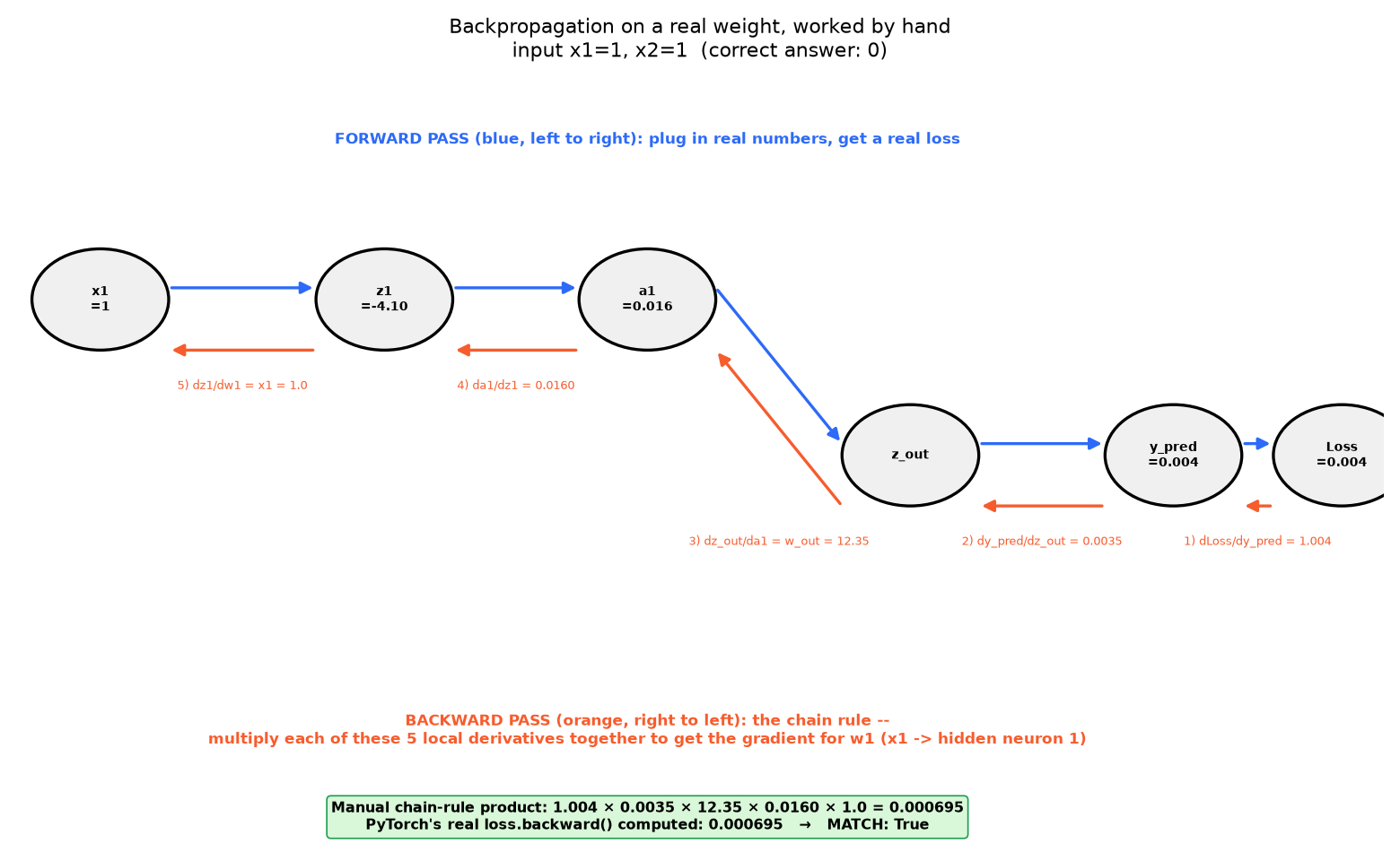
They match exactly — 0.000695 both ways — because they're the same calculation. PyTorch's
autograd isn't doing anything conceptually different from this five-line hand derivation; it's just doing
it automatically, for every single one of the network's weights, every training step.
🧩 AI Architectures
A quick-reference guide to the major deep learning architectures — what each one is structurally, its key properties, and what it's actually used for today. Companion to the AI Debate timeline, which covers how and why these ideas developed historically; this page is the fast lookup table.
The Three Types of Machine Learning
Every architecture below is a structure for implementing one of these three learning paradigms — the paradigm determines what kind of problem and what kind of data a model is built for; the architecture (MLP, CNN, Transformer, etc.) is just the specific mechanism used to do it.
📍 Supervised Learning
Learns a mapping from labeled input→output pairs — every training example comes with the "correct answer" attached.
- Classification — sorting into discrete categories (spam / not spam, cat / dog)
- Regression — predicting a continuous value (house price, temperature)
- 🧩 MLP, CNN, RNN, LSTM, Transformer — all trained this way by default
🔍 Unsupervised Learning
Finds structure in unlabeled data — there's no "correct answer" given; the model has to discover patterns on its own.
- Clustering — grouping similar items (e.g. K-means for customer segmentation)
- Dimensionality reduction — compressing data down to its essential structure (e.g. PCA, autoencoders)
- 🧩 GANs and diffusion models — both learn a data distribution with no labels
🎮 Reinforcement Learning
An agent takes actions in an environment and learns from the rewards (or penalties) that follow — no labeled dataset at all, just trial and error.
- Policy learning — deciding which action to take in a given state
- Value estimation — predicting how good a state/action actually is long-term
- 🧩 Classic use: game-playing agents, robotics
- 🧩 Modern use: RLHF — how ChatGPT and other LLMs get fine-tuned on human preferences (see the 2022 ChatGPT entry in AI Debate)
MLP
Fully connected feedforward network. Every neuron in one layer connects to every neuron in the next; information moves in a single direction from input to output.
- Fully connected ("dense") layers
- Universal function approximator given enough hidden units
- No built-in assumptions about spatial or sequential structure
- Prone to overfitting on high-dimensional raw input
- Common activations: ReLU, sigmoid, tanh
- 📊 Tabular data classification / regression
- 🧪 Baseline models
- 🔍 Simple pattern recognition
CNN
Uses learned convolutional filters to extract spatial features from images, then pools and flattens them into a final classifier.
- Local receptive fields extract spatial features
- Weight sharing across the whole image (few parameters per filter)
- Pooling layers add translation tolerance
- Hierarchical: early layers learn edges, deeper layers learn shapes/objects
- 🖼️ Image classification
- 🎯 Object detection
- ✂️ Image segmentation
- 👁️ Computer vision generally
RNN
Loops information from each step forward into the next, so the network's output depends on everything it has seen so far in the sequence.
- Hidden state carries information across time steps
- Shares the same weights at every step
- Handles variable-length sequences natively
- Struggles with long-range dependencies (vanishing/exploding gradients)
- 📈 Short time-series prediction
- 🔤 Simple sequence modeling
- 🧩 Teaching the concept behind LSTM/GRU (largely superseded by them in practice)
LSTM
An RNN variant with a separate cell state and three gates that learn what to keep, discard, and output — solving the vanishing-gradient problem plain RNNs suffer from.
- Dedicated cell state (Cₜ) acts as a long-term memory highway
- Forget, input, and output gates control information flow
- Mitigates vanishing gradients over long sequences
- More parameters and slower to train than a plain RNN or GRU
- 🌐 Machine translation
- 📝 Text summarization
- 💬 Sentiment analysis
- 📊 Time-series forecasting
GRU
A simplified LSTM that merges the cell and hidden states into one, using just two gates (reset and update) instead of three.
- Only two gates (reset, update) — no separate cell state
- Fewer parameters than LSTM
- Often trains faster than LSTM; comparable accuracy on many tasks
- Still captures long-range dependencies via the update gate
- 🔤 Text generation
- 🎙️ Speech recognition
- 📊 Time-series analysis
- 🔮 Sequence prediction
Transformer
Replaces recurrence entirely with a self-attention mechanism that weighs the importance of every token against every other token in the sequence, all at once.
- Self-attention: every position attends to every other position directly
- No recurrence — fully parallelizable across the sequence during training
- Captures long-range dependencies without a vanishing-gradient penalty
- Scales well with more data and compute (the basis of modern foundation models)
- 🏛️ Foundation models (BERT, GPT)
- 🌐 Machine translation
- 🔤 Text generation
- 🖼️ Vision Transformers (ViT)
Autoencoder
Squeezes the input down through a bottleneck into a compressed latent representation, then reconstructs the original from that compressed form.
- Unsupervised — trained to reconstruct its own input, no labels needed
- Bottleneck layer forces a compressed ("latent") representation
- Reconstruction error itself is a useful signal
- Vanilla autoencoders compress; variants (VAE) are needed to generate new samples
- 📉 Dimensionality reduction
- 🚨 Anomaly detection (via reconstruction error)
- 🧹 Image denoising
- 🎯 Recommender systems
🔬 CNN Deep Dive: The Math + Code Behind Convolution
The CNN card above shows the concept. Here's the actual pipeline worked through by hand — the operation each stage performs, a from-scratch implementation, and a verified numeric example run through it end to end.
Each output pixel of a conv layer is a weighted sum of the input patch under the filter, plus a bias. Frameworks call this "convolution," but it's technically cross-correlation — the kernel isn't flipped, unlike the textbook-strict definition of convolution:
ReLU zeroes out negative activations — cheap to compute, and it's what makes deep stacks of these layers trainable:
Max pooling slides a window over the feature map and keeps only the strongest activation in each region, which shrinks the map and adds a little translation tolerance:
def conv2d(x, kernel, bias=0.0):
    H, W = x.shape
    kh, kw = kernel.shape
    out = np.zeros((H - kh + 1, W - kw + 1))
    for i in range(out.shape[0]):
        for j in range(out.shape[1]):
            patch = x[i:i+kh, j:j+kw]
            out[i, j] = np.sum(patch * kernel) + bias
    return out

def relu(x):
    return np.maximum(0, x)

def max_pool2d(x, size=2, stride=2):
    H, W = x.shape
    oh, ow = H // stride, W // stride
    out = np.zeros((oh, ow))
    for i in range(oh):
        for j in range(ow):
            r, c = i * stride, j * stride
            out[i, j] = np.max(x[r:r+size, c:c+size])
return outA 6×6 input, a 3×3 vertical-edge kernel, bias −1 — run through conv2d → relu → max_pool2d exactly as defined above:
3 0 4 1 2 5
1 2 0 3 4 1
4 1 3 0 1 2
0 3 2 4 0 3
2 4 1 0 3 1
1 0 3 2 4 0
 1  0 -1
 1  0 -1
 1  0 -1
 0 -2 -1 -5
-1 -2 -1  0
-1  3  1 -3
-4  0 -2  1
0 0 0 0
0 0 0 0
0 3 1 0
0 0 0 1
0 0
3 1
🔬 Transformer Deep Dive: Scaled Dot-Product Attention
The Transformer card above shows the block diagram. Here's the actual mechanism inside "Multi-Head Attention" — how Q, K, and V turn into an output vector per token, worked through by hand on 3 toy tokens.
Every token projects into a Query, Key, and Value vector via learned weight matrices. Each token's Query is dotted against every token's Key to get a similarity score, scaled down so the softmax doesn't saturate into near-one-hot at large dimensions:
In practice this is run h times in parallel on smaller projected slices ("heads"), each free to specialize on a different kind of relationship, then the results are concatenated and mixed back down with one more learned matrix:
Since there's no recurrence, the model has no inherent sense of token order — position has to be injected explicitly, added directly onto the input embeddings before the first layer:
def softmax(x, axis=-1):
    x = x - np.max(x, axis=axis, keepdims=True)
    e = np.exp(x)
    return e / np.sum(e, axis=axis, keepdims=True)

def scaled_dot_product_attention(Q, K, V):
    d_k = Q.shape[-1]
    scores = Q @ K.T / np.sqrt(d_k)
    weights = softmax(scores, axis=-1)
    output = weights @ V
    return output, weights

# one head: project tokens to Q, K, V first
Q = X @ W_Q
K = X @ W_K
V = X @ W_V
out, weights = scaled_dot_product_attention(Q, K, V)3 toy tokens, d_model = 4, single head. X is the input embeddings; W_Q/W_K/W_V are fixed toy projection weights (normally learned). Note every attention-weight row sums to exactly 1 — that's the softmax normalization working as intended.
1 0 1 0
0 2 0 1
2 1 0 0
2 0 1 1
0 3 2 1
2 1 1 2
0 1 1 2
3 1 2 0
1 2 1 2
3 2 0 1
0 2 5 2
4 1 2 2
1.5 4.0 2.5
3.5 3.5 5.0
3.0 4.5 4.5
0.063 0.766 0.171
0.154 0.154 0.691
0.100 0.450 0.450
0.872 1.829 4.173 1.937
3.229 1.309 2.154 1.846
2.100 1.550 3.149 1.900
Diagrams are simplified for clarity, not full circuit/data-flow specs. For the historical "why" behind these — who invented what, and what problem each one solved — see the AI Debate timeline.
🔬 Silicon & Transistor Design
How a bare silicon wafer becomes a working transistor, how transistors combine into logic, and how the transistor's own shape has evolved (planar → FinFET → GAAFET) to keep scaling working. Companion to AI Architectures — same "fast lookup" spirit, different layer of the stack. Timeline first, then the quick-reference cards below.
A History of the Transistor and the Integrated Circuit
Band Theory of Solids — Alan Wilson
Before there could be a transistor, there had to be a reason to believe a "semiconductor" was a real, useful category of material rather than just an unreliable in-between. Cambridge physicist Alan Wilson, working at Werner Heisenberg's institute in Leipzig, adapted the quantum-mechanical band theory Felix Bloch and Rudolf Peierls had been developing for crystalline solids into a model explaining why semiconductors behave the way they do — filled and empty energy bands, "forbidden" band gaps between them, and vacancies in a nearly-full band that act as mobile positive charge carriers (the theoretical origin of the "hole," a term this entire page has used constantly). Wilson's papers essentially founded solid-state physics as a recognized field on their own. The 15 years between this and 1947 were spent on the unglamorous but essential work of learning to purify and precisely dope silicon and germanium — without which none of the following history happens.
The Point-Contact Transistor — Bardeen & Brattain, Bell Labs
The first working transistor, ever. A crude germanium device with two closely-spaced metal point contacts pressed into the surface — fragile, hard to manufacture, but it proved solid-state amplification could replace vacuum tubes. Shockley wasn't part of the actual invention, and was reportedly frustrated by that — which pushed him toward the next entry.
The Junction Transistor — William Shockley
Shockley worked out the theory for a far more practical, manufacturable design: a three-layer sandwich of alternating doped silicon — NPN or PNP — instead of fragile point contacts. This is the structural ancestor of the BJT (bipolar junction transistor) still used today, and the reason "NPN"/"PNP" became the standard shorthand for bipolar transistor polarity.
First Silicon Transistor — Gordon Teal, Texas Instruments
Everything up to this point was germanium. Silicon is harder to purify and work with, but far more thermally stable — germanium transistors degraded badly in heat. TI's silicon transistor set the entire industry on the material path it's still on 70+ years later.
Nobel Prize in Physics — Shockley, Bardeen & Brattain
Jointly awarded "for their researches on semiconductors and their discovery of the transistor effect."
The Shockley 4-Layer Diode, and the "Traitorous Eight"
Shockley's own company (Shockley Semiconductor Laboratory) developed the Shockley diode — a distinct device from the transistor: a 4-layer PNPN structure (vs. the transistor's 3 layers) that latches into an on/off state with no ongoing control input, the conceptual ancestor of the thyristor/SCR. The same year, eight of Shockley's own engineers — unable to tolerate his management style — quit to found Fairchild Semiconductor, effectively founding the culture of Silicon Valley as a place engineers leave to start competitors.
The First Integrated Circuit — Jack Kilby, Texas Instruments
Kilby built the first working IC: multiple components (transistor, resistors, capacitor) on one piece of germanium — but connected by fine external "flying wires" soldered by hand, not yet mass-producible. He won the Nobel Prize in Physics for it in 2000.
The Planar Process & the Monolithic IC — Hoerni & Noyce, Fairchild
Jean Hoerni's planar process (an oxide layer grown over the whole silicon surface, then selectively etched) let Robert Noyce design an IC with components connected by printed metal traces directly on the chip — no wires at all. This is the version that could actually be mass-produced, and it's the direct ancestor of every chip made since. Noyce and Kilby are jointly credited as IC co-inventors, arrived at independently within months of each other.
The First MOSFET — Atalla & Kahng, Bell Labs
Fabricated in November 1959, patents filed March 1960. Mohamed Atalla had been working on a persistent problem — unstable "surface states" on silicon — and found that growing a clean thermal silicon-dioxide layer suppressed them enough to build a reliable field-effect transistor. This is the literal origin of "MOS" in NMOS/PMOS/CMOS, and arguably the single most consequential invention in this whole timeline — MOSFETs are, by unit count, the most manufactured device in human history.
CMOS Invented — Frank Wanlass & Chih-Tang Sah, Fairchild
Showed that pairing a P-channel and N-channel MOS transistor in the complementary configuration drew almost zero standby power. Barely noticed at the time — bipolar logic was faster and dominant — but this exact idea is why virtually every digital chip made today can run cool enough, and battery-efficient enough, to exist at all.
Moore's Law — Gordon Moore
Moore (soon a Fairchild/Intel co-founder) observed that the number of components on a chip was roughly doubling every year, and predicted it would keep going. Later revised to ~every two years. Not a law of physics — a self-fulfilling industry roadmap that shaped decades of R&D investment.
DRAM Invented — Robert Dennard, IBM
Working on MOS memory at IBM's Watson Research Center, Dennard realized a single transistor and a single capacitor were enough to store one bit — the capacitor holds the charge (the "1" or "0"), the transistor controls reading and writing it. IBM filed the patent in 1967 (granted 1968). This one-transistor-one-capacitor cell is still, unchanged in principle, how essentially all of main system memory works today — dramatically denser than the magnetic-core memory it replaced.
The Floating-Gate Memory Effect — Kahng & Sze, Bell Labs
Dawon Kahng (co-inventor of the MOSFET itself, 8 years earlier) and Simon Sze discovered that a transistor gate fully isolated by insulation on all sides could still be made to hold a trapped electrical charge — and that charge would stay put with the power off, for years, while still being erasable and reprogrammable. This is the physical basis of every non-volatile memory that followed: PROM, EPROM, EEPROM, and eventually Flash. Unlike DRAM's capacitor (which leaks charge in milliseconds and must be constantly refreshed), a floating gate holds its charge with no power at all.
Intel Founded, Then the First Microprocessor
Noyce and Moore left Fairchild to found Intel in 1968. In 1971, Intel shipped the 4004 — the first commercially available complete CPU on a single chip, originally built for a Japanese calculator company, Busicom. The idea of "a computer on one chip" started here.
Flash Memory Invented — Fujio Masuoka, Toshiba
Masuoka led a small, semi-secret project at Toshiba to build a memory chip based on the floating-gate effect (1967) that could store far more data, affordably, than existing EEPROMs. The key trick: unlike EEPROM, which erases and rewrites one byte at a time, this new memory could erase entire blocks at once — much faster, much simpler circuitry. His colleague Sho-ji Ariizumi suggested the name "flash," because the block-erase process reminded him of a camera flash going off.
NAND Flash — Fujio Masuoka, Toshiba
Masuoka's original 1980 design is what's now called NOR flash — fast random access, but each cell needs its own direct wiring connection, capping density. At the 1987 IEDM conference, he introduced NAND flash: cells wired in series instead of parallel, trading random-access speed for dramatically higher density and lower cost per bit. NAND's density-over-speed tradeoff is exactly why it became the basis for essentially all bulk flash storage — USB drives, SD cards, and eventually SSDs — while NOR stuck to smaller, latency-sensitive uses like storing a device's boot firmware.
Copper Interconnects — IBM
IBM's damascene process replaced aluminum wiring with copper — lower resistance, faster chips — solving the problem that copper can't be dry-etched the way aluminum can (etch a trench first, then fill it with copper, instead).
High-k Metal Gate Goes Commercial — Intel 45nm
Plain silicon dioxide gate oxide had gotten down to just a few atoms thick and started leaking current via quantum tunneling. Intel's 45nm node was the first to ship a high-k dielectric (hafnium-based) paired with a metal gate at real volume, buying scaling several more nodes of headroom.
FinFET Goes Commercial — Intel 22nm "Tri-Gate"
The transistor channel goes 3D for the first time in mass production — a vertical "fin," gated on three sides instead of one — specifically to fix the leakage problems planar transistors were suffering below ~20nm.
3D NAND — Samsung
Planar NAND hit the same wall every planar structure on this timeline eventually hits: cells packed close enough together started interfering with their neighbors' stored charge. Samsung's answer was the same one this page keeps returning to — go vertical. V-NAND stacked memory cells in layers rising out of the wafer instead of spreading them across it, the direct ancestor of today's 100+ layer 3D NAND that underlies essentially all SSD storage (see the 3D Die Stacking card).
HBM Standardized, Then Shipped — JEDEC / SK Hynix / AMD
JEDEC published the HBM standard (JESD235) in October 2013, co-developed by AMD, SK Hynix, and Samsung; SK Hynix produced the first HBM chip that same year. The first product to actually use it: AMD's Radeon R9 Fury X (Fiji GPU), 2015 — stacked DRAM on a 2.5D silicon interposer, 512 GB/s of bandwidth at a fraction of GDDR5's power draw. This is the same HBM that's now essential to every high-end AI accelerator.
Chiplets Go Mainstream — AMD Zen 2 / Ryzen 3000
Instead of one large monolithic die, AMD shipped consumer CPUs built from several smaller "chiplets" wired together — separating the (expensive, harder to yield) CPU cores from the (cheaper, older-process) I/O die. A direct response to monolithic scaling getting more expensive per generation, and the conceptual bridge to today's 2.5D/3D packaging era.
GAAFET Goes Commercial — Samsung 3nm (MBCFET)
The channel is reshaped again, from a vertical fin into horizontal stacked nanosheets, with the gate now wrapping all four sides instead of three — the next answer to the same leakage problem FinFET solved a decade earlier, now recurring at a smaller scale.
The Present — GAAFET at Volume, Hybrid Bonding Everywhere
Intel's 18A (RibbonFET) and TSMC's N2 (Nanosheet GAA) both reached high-volume production. HBM is moving to hybrid bonding starting at HBM4E/HBM5 to push past 16-layer stacks. TSMC alone is targeting 100,000–120,000 wafers/month of advanced packaging capacity by the end of 2026 — 3D stacking has gone from a research curiosity to one of the industry's primary growth levers.
Quick Reference — How Each Piece Actually Works
Materials & Fabrication Process
Silicon Doping
Silicon has 4 valence electrons per atom, bonded to 4 neighbors. Swap in a trace 5-electron atom (phosphorus, arsenic) and you get one leftover free electron — N-type. Swap in a 3-electron atom (boron) and one bond is left incomplete — a mobile "hole" — P-type.
- Dopant concentration: ~1 per million–billion silicon atoms (standard); much higher ("n+"/"p+") for low-resistance contacts
- Done via ion implantation (fire ions in, then anneal) or thermal diffusion
- Donors (N-type) vs. acceptors (P-type) — the terms describe giving vs. taking an electron
Photolithography
The step that makes everything else possible: printing the circuit's pattern onto the wafer using light. It doesn't modify the silicon itself — it creates a precise stencil (patterned photoresist) that determines exactly where the next step (etching or ion implantation) is allowed to act.
- Coat wafer with light-sensitive photoresist → soft bake
- Align & expose through a patterned mask/reticle (in an ASML-style scanner)
- Develop — dissolves either the exposed or unexposed resist, leaving a stencil
- Etch or implant through the stencil, then strip the resist — repeat for every layer
- 🔬 Feature size is limited by light wavelength (diffraction) — shrinking transistors forced a jump from 193nm DUV to 13.5nm EUV light
- ⚙️ EUV is absorbed by nearly everything, including air — the whole optical path runs in vacuum with mirrors instead of lenses
Ion Implantation
The actual machine-level process behind doping (card 1): dopant atoms are ionized, electrically accelerated to a precise energy, and fired directly at the wafer. The photoresist stencil from lithography blocks them everywhere except the intended openings — then an anneal (brief high-heat step) repairs the crystal lattice damage and moves the dopants into proper lattice positions so they're electrically "activated."
- Implant energy controls depth; dose (ion count) controls concentration
- Dominant technique in modern fabs — tighter control than the older alternative, thermal diffusion (heating the wafer in a dopant-rich gas and letting atoms diffuse in)
- Same stencil-then-modify pattern as etching — implantation is doping's version of it
Etching
The other thing the lithography stencil enables: selectively removing material. Wet etch (chemical bath) is cheap but isotropic — it eats sideways under the mask as fast as it eats downward, limiting precision. Dry/plasma etch (reactive ion bombardment) is anisotropic — it etches almost straight down, reproducing the mask shape precisely, which is why it's the standard for anything below a few microns.
- Every trench, via, and gate structure in the IC layer stack is cut this way, through a fresh resist stencil each time
- Selectivity matters: the etch chemistry must attack the target material much faster than the resist or underlying layers
- Strip the resist afterward — same "coat → pattern → modify → strip" cycle as ion implantation
Thin-Film Deposition
How the actual material layers in the IC stack get built up. CVD (Chemical Vapor Deposition) flows reactive gases over the wafer, where they chemically react and deposit a film right at the surface — it coats contours evenly ("conformal"), good for oxides and some metals. PVD (Physical Vapor Deposition / sputtering) bombards a solid target with ions, physically knocking atoms free to travel in straight lines and land on the wafer — more directional, commonly used for metal layers and barrier films.
- ALD (Atomic Layer Deposition) — a slower, even more precise CVD variant — builds up film one atomic layer at a time, used for today's high-k gate dielectrics
- Choice of method depends on the material and how conformal the coating needs to be
- Every layer in the IC layer stack — oxide, metal, barrier, dielectric — got there via one of these methods
CMP — Planarization
Chemical Mechanical Planarization — a rotating pad plus an abrasive/chemical slurry that grinds each freshly-deposited layer perfectly flat before the next lithography step. This isn't cosmetic: photolithography has an extremely shallow depth of focus, so any leftover bumps from the previous layer would blur the next pattern out of focus.
- Runs after essentially every deposition step in the BEOL (metal/dielectric) stack
- Also essential to copper's damascene process — CMP is what removes the excess copper deposited everywhere, leaving it only in the etched trenches
- Without CMP, multi-layer copper interconnects (8–15+ layers) simply wouldn't be manufacturable
IC Layer Stack
Bottom-up: FEOL (front-end-of-line) builds the transistors themselves — substrate, wells, gate stack, contacts. BEOL (back-end-of-line) is pure wiring above that — 8–15+ stacked copper layers separated by insulating dielectric, connected by vias.
- SiO₂ gate oxide → high-k (HfO₂): plain SiO₂ got too thin (atoms-thick) and started leaking
- Polysilicon gate → metal gate: avoids "poly depletion" robbing capacitance at small scale
- Aluminum → copper wiring (1997, IBM's damascene process): lower resistivity, needs a Ta/TaN barrier since Cu diffuses into silicon
Device Structures & Logic
Bipolar Junction Transistor — NPN / PNP
Three doped regions in a row — N-P-N (shown) or P-N-P — instead of a FET's source/gate/drain. A small current injected into the thin middle Base region controls a much larger current flowing Collector→Emitter. This is the key structural difference from NMOS/PMOS next door: a BJT is current-controlled, a MOSFET is voltage-controlled (the gate draws essentially no current at all, just an electric field).
- NPN conducts Collector→Emitter when base current flows into the base; PNP is the mirror image, conducting Emitter→Collector when current flows out of the base
- The Base must be thin and lightly doped relative to Emitter/Collector — that asymmetry is what lets a small base current control a disproportionately larger collector current (current gain, "beta")
- This was the only transistor type that existed from 1947 (Bardeen & Brattain's point-contact device) through the invention of the MOSFET in 1959–60 — every "transistor" milestone on this page's timeline before 1959 is a BJT
A BJT is always drawing some base current to stay on, which burns power continuously — fine for a handful of transistors, ruinous for billions of them switching on a single die. A MOSFET's gate is capacitive: once charged, it draws essentially zero steady current. CMOS logic (card 10) needs that near-zero static power to scale to modern transistor counts. BJTs never disappeared, though — they're still the default choice for analog amplification, RF power stages, and voltage regulators, anywhere raw current-handling and gain matter more than density.
NMOS Transistor
N+ source and drain sit in a P-type body. Positive gate voltage attracts electrons to form a conductive channel beneath the gate, letting current flow source→drain. Zero gate voltage = no channel = off.
- Two built-in p-n junctions: source↔body and drain↔body — the "body diodes"
- Body is tied to ground (most negative rail) to keep those diodes reverse-biased/off
- Conducts when gate is high
- Only turns on once gate voltage clears a threshold voltage (VT) — below it, essentially no channel forms at all; this threshold is itself tuned by the doping concentration in the body
Electrons (the carriers NMOS relies on) have significantly higher mobility through silicon than holes (what PMOS relies on) — they simply move faster through the lattice for the same electric field. That's a real, physical asymmetry between the two transistor types, not just a labeling convention, and it's the direct cause of the PMOS sizing note in the next card.
PMOS Transistor
Mirror image of NMOS: P+ source/drain in an N-type well. Negative gate voltage (relative to source) attracts holes to form the channel — so PMOS conducts when the gate is low, the opposite of NMOS.
- Same two body-diode junctions as NMOS, polarity reversed
- N-well is tied to VDD (most positive rail) to keep them reverse-biased/off
- Conducts when gate is low — exact complement of NMOS
Because holes move slower than electrons (previous card), a PMOS device with the same physical dimensions as its NMOS partner would pull current more weakly and switch more slowly — an asymmetric, imbalanced gate. Chip designers compensate by making the PMOS transistor's channel wider than the paired NMOS (often ~2× in older processes, less at advanced nodes) so both halves of a CMOS gate switch at roughly matched speed. This is a real, physical layout decision on every standard-cell library, not a rounding detail.
CMOS Inverter
The simplest CMOS gate: one PMOS (pull-up, wired to VDD) and one NMOS (pull-down, wired to GND), gates tied together as the input. IN=0 → PMOS on/NMOS off → OUT=1. IN=1 → NMOS on/PMOS off → OUT=0. Only one device conducts at a time.
- ⚡ Near-zero static current — draws power only while switching, not while idle
- 🧩 Same principle scales to any logic gate (NAND, NOR, etc.), not just an inverter
- 🏭 The circuit-level standard since the 1980s–90s, unchanged even as the transistor shape (planar→FinFET→GAAFET) has changed underneath it
"Near-zero static current" hides one real transient cost: during the brief moment a gate is actually switching, the input voltage passes through a middle range where both the NMOS and PMOS are partially conducting at once — briefly punching a direct, unwanted path from VDD straight to GND. This is called short-circuit (or "crowbar") current, and it's a real contributor to a modern chip's total dynamic power draw, alongside the far larger cost of simply charging/discharging each wire's capacitance on every transition. It's also why input signals with a slow, lazy rise/fall time are worse for power than sharp, fast-switching ones — the slower the transition, the longer both transistors sit in that partially-on crossover zone.
Logic Gates from Transistors
The inverter's pull-up/pull-down pattern extends directly to any gate: mirror the pull-down network's series/parallel wiring into the pull-up network (swapped), and NMOS/PMOS logic stays complementary. NAND and NOR are the two "universal" gates — every other digital function (AND, OR, XOR, adders, muxes, flip-flops, entire CPUs) is built by wiring more of these two primitives together at massive scale.
- Series in the pull-down (NMOS) network ⇄ parallel in the pull-up (PMOS) network, and vice versa
- AND = NAND + inverter; OR = NOR + inverter — the "positive" gates cost one extra transistor pair
- An N-input NAND/NOR just adds more transistors in the same series/parallel pattern — no new principle needed
Transistor Shape Evolution: Planar → FinFET → GAAFET → CFET
Same materials at every stage — silicon, a thin dielectric, and a conductive gate — the only thing that changes generation to generation is the geometry: how many faces of the channel the gate material can physically touch. More contact = more electrostatic control = less leakage when "off," which is the entire reason each transition happened.
- Planar → FinFET (2011): below ~20nm, a single flat gate face couldn't fully shut the channel off — leakage got too severe. Standing the channel up into a fin let the gate wrap 3 faces instead of 1.
- FinFET → GAAFET (2022+): the same leakage problem recurred once FinFET itself got small enough — fin height/width became hard to manufacture reliably. Laying the channel down into stacked horizontal sheets let the gate wrap all 4 faces, plus each sheet's width can now be tuned individually (unlike a fin's fixed height).
- GAAFET → CFET (beyond 2nm, published roadmap): instead of reshaping the channel again, stack an NMOS GAAFET directly on top of a PMOS GAAFET in the same horizontal footprint — the CMOS pair (card 10) that used to sit side-by-side now sits vertically, doubling density without shrinking anything.
- What never changes: NMOS/PMOS doping, the CMOS wiring principle, and the basic source/gate/drain roles — only the channel's physical shape and how much of it the gate can touch.
The Scaling Endgame — From 10µm to the Atomic Limit
For the first ~35 years, the "node name" (10µm, 3µm, 1µm...) was the transistor's actual gate length, measured directly. That stopped being true starting around Intel's 0.25µm process (1997), whose real gate length was already 0.20µm — smaller than the name on the label. The divergence then got dramatic: at the 45nm node (2007), Intel's actual gate length hit ~25nm and effectively stopped shrinking — after the 32nm node, gate length was even briefly increased rather than shrunk further. FinFET (2011) locked gate length in as roughly constant from there on, since its density gains come from fin geometry, not a shorter gate. So for essentially the entire FinFET/GAAFET era, the one dimension the node name used to literally describe hasn't meaningfully changed at all — everything since has been about squeezing transistors and wires closer together, not making the gate itself shorter. By the time you reach "22nm," "14nm," "10nm," "7nm" and beyond, the node name is a generational marketing label, not a measurement of any specific physical feature — different foundries' "7nm" processes aren't even directly comparable to each other in actual transistor density.
If not gate length, what's real underneath the label? Two genuinely measurable pitches: Contacted Gate Pitch (CGP) — the smallest distance between adjacent transistor gates — and Metal Pitch (MP) — the smallest spacing between wires on the finest interconnect layer. Industry convention loosely ties the node name to about half the metal pitch (a "5nm"-class chip ≈ 15nm half-pitch, "3nm"-class ≈ 12nm, "1nm"-class ≈ 8nm) — but that's a per-company convention, not a binding formula, which is exactly why Samsung was able to rebrand a second-generation "3nm-class" process as "2nm" without a fundamentally different underlying jump in either pitch. Because of this ambiguity, IEEE's International Roadmap for Devices and Systems (IRDS) has proposed retiring the single "nm" label entirely in favor of reporting G-M-T directly: Gate pitch, Metal pitch, and number of device Tiers. A current "5nm"-class chip, reported honestly, would be something like G48M36T1 (48nm gate pitch, 36nm metal pitch, 1 tier of devices) — and that last "T" is about to matter a lot more, since CFET (next section) makes "how many tiers of transistors stacked on each other" a real, separate axis for the first time.
- Quantum tunneling: once a barrier (like a gate oxide) gets down to just a few atoms thick, electrons can pass straight through it even though classical physics says they shouldn't have enough energy to — this is exactly why plain SiO₂ gate oxide had to be replaced with high-k dielectrics (card 7), and it recurs at every subsequent shrink.
- Random dopant fluctuation: a transistor's channel at advanced nodes contains only a small, countable number of dopant atoms — sometimes just a few dozen. Since doping is a statistical process (ion implantation, card 3), the exact count and position varies transistor to transistor, and at small enough scale that random variation becomes a bigger effect on behavior than the intended design — a real manufacturing yield and uniformity problem, not just a theoretical one.
- The hard floor: silicon's own crystal lattice has a fixed spacing of about 0.54nm between repeating units (a single silicon atom's covalent radius is about 0.11nm). A "2nm" process is already only about 4 silicon atoms wide in its smallest real dimensions. You cannot make a silicon transistor smaller than a handful of atoms and still have it behave like a controllable switch — single-atom transistors have been built in research labs, but nothing about them is stable, uniform, or manufacturable at the billions-per-chip scale this entire page has been about.
CFET (Complementary FET) is the industry's actual, published roadmap answer for what comes after GAAFET — not speculation. Instead of shrinking the transistor further, CFET stacks an NMOS GAAFET directly on top of a PMOS GAAFET in the same horizontal footprint, doubling density again without needing the channel itself to get any smaller. It's the same "go vertical instead of smaller" move this page has now seen twice already — FinFET's fin, GAAFET's stacked sheets, 3D NAND's stacked cells (timeline, 2013), and now CFET stacking the two transistor types themselves.
Once you're genuinely out of room to shrink a silicon switch, the research directions split into two different strategies:
- 🔬 New channel materials: 2D materials like graphene or single-atomic-layer transition-metal dichalcogenides (e.g. molybdenum disulfide) can in principle form a working transistor channel that's a single atom thick — actively researched, not yet manufacturable at scale
- 🧪 Different computing paradigms entirely — several of which are already on this page: analog compute (card 15, "Unconventional AI"), optical/photonic (card 16), and thermodynamic computing (card 16) all sidestep the "keep shrinking a classical digital switch" race rather than trying to win it
- ⚛️ Quantum computing is the most radical version of that same idea — rather than a smaller classical bit, use a quantum state (superposition/entanglement) as the unit of computation itself, which doesn't run into "the atomic limit" the same way at all since it's not trying to be a tiny version of a transistor
Assembly & Packaging
3D Die Stacking
Instead of one flat die, stack multiple dies vertically and connect them with vertical TSVs (through-silicon vias, drilled straight through the silicon) or hybrid bonding (direct copper-to-copper bonds at the wafer level, even finer pitch than TSVs).
- 🧠 HBM — stacked DRAM in every high-end AI GPU (NVIDIA, AMD Instinct)
- 💾 3D NAND — 100+ stacked memory-cell layers, effectively all SSD storage today
- 🎮 AMD 3D V-Cache — extra L3 cache die stacked directly on Ryzen CPU dies
- 🏭 Intel Foveros — 3D stacking used in shipping Meteor Lake-class chips
- 📈 TSMC targeting 100,000–120,000 wafers/month of advanced packaging capacity by 2026
CoWoS vs. EMIB — Two Ways to Wire Chiplets Together
CoWoS (Chip-on-Wafer-on-Substrate) puts a full silicon interposer underneath the entire package — every die sits on top of one continuous, high-density silicon layer. EMIB (Embedded Multi-die Interconnect Bridge) skips the interposer almost entirely — it embeds a small silicon "bridge" chiplet into the organic package substrate only at the exact spot where two dies need a dense connection, and everywhere else the dies just sit on ordinary (cheaper) substrate.
- Reticle-size scaling: EMIB-M already at 6×, projected 8–12× by 2026–27, vs. CoWoS-S at 3.3× and CoWoS-L at ~3.5× today (TSMC targeting a 14-reticle CoWoS by 2028)
- Panel utilization: Intel cites ~90% for EMIB vs. ~60% for CoWoS — EMIB wastes less material per package
- Cost: EMIB is generally cheaper — no full interposer to fabricate
- Track record: CoWoS is the proven, dominant backbone of the current AI boom — it's what NVIDIA's GPUs actually ship on today
Honestly — neither, cleanly. They're different architectural bets, not a better/worse pair:
- 🏆 CoWoS wins on proven scale — it's carried the entire AI GPU boom so far, at higher absolute interconnect density per package
- 🏆 EMIB wins on cost, utilization, and near-term scaling headroom — cheaper per package, less wasted material, and currently ahead on reticle-size scaling trajectory
- ⚖️ The actual 2026 story isn't "EMIB beat CoWoS" — it's dual-sourcing: TSMC's CoWoS capacity is capacity-constrained (real demand exceeds real supply), so major customers are qualifying EMIB as a second source rather than picking a winner. MediaTek is reportedly using both; Google's reported 9th-gen TPU move and NVIDIA's reported interest in EMIB for its Feynman chips are read as capacity-driven diversification, not a verdict that EMIB is technically better.
Frontier Architectures
Unconventional AI Silicon — One Assumption Each Eliminates
A standard GPU makes several load-bearing assumptions at once: weights live in off-chip DRAM/HBM, big models need multiple interconnected dies, compute and memory are physically separate, the server is built compute-centric (a little memory around a lot of compute), the chip must be general-purpose, digital circuits must switch discretely and synchronously, and it all has to be made on a $150–400M EUV scanner. Every company below picks exactly one of those assumptions and deletes it — the table is organized by what problem they're attacking, not by who's raised the most money.
| Company | The problem it attacks | The technology |
|---|---|---|
| Groq | Off-chip memory (DRAM/HBM) is slow and power-hungry to keep feeding a GPU's compute units — the "memory wall" | All-SRAM weight storage (no DRAM at all) + fully deterministic, compiler-scheduled execution — no runtime scheduler, so there's nothing unpredictable left to cause a stall |
| Cerebras | Lithography's reticle limit forces big chips to be built from many small dies, wired together with lossy, power-hungry interconnect | Wafer-Scale Engine — treats an entire 300mm wafer as one chip, with redundant cores/routing engineered in to tolerate the fabrication defects that would normally kill a chip this large |
| d-Matrix | Every multiply-accumulate operation requires shuttling data between separate compute and memory chips — the classic "von Neumann bottleneck" | Digital In-Memory Compute — embeds the actual multiply-accumulate logic directly inside the SRAM bit cells, so computation happens exactly where the data already sits |
| Fractile | Same von Neumann bottleneck as d-Matrix, different implementation | Its own take on in-memory inference compute, UK-based |
| SambaNova | A GPU's pipeline is fixed in silicon — software has to contort itself to fit the hardware, not the other way around | Reconfigurable Dataflow Unit — the hardware itself reconfigures per model, fusing many operations into one pass; a 3-tier SRAM/HBM/DDR5 hierarchy keeps "hot" data close and "cold" data cheap |
| NextSilicon | Fixed CPU/GPU architectures can't adapt to a program's actual runtime behavior | "Software-defined" hardware that profiles a workload as it runs and reconfigures its own dataflow routing to match — aimed at HPC as much as AI |
| Positron / Majestic Labs | Servers are built compute-first with a little memory bolted on — but modern LLMs are increasingly memory-capacity-bound, not compute-bound | "Memory-first" design: Positron's Archer ASIC prioritizes bandwidth per watt; Majestic disaggregates memory from compute entirely, targeting ~100× the usable memory pool of a normal GPU server |
| Etched (Sohu) | A GPU's generality (any workload, any architecture) costs real efficiency — GPU FLOP utilization on inference often falls to 30–40% | Hard-codes the transformer computation graph itself into fixed-function silicon — runs any transformer model, but nothing else, eliminating instruction-scheduling/kernel-launch overhead entirely |
| Taalas | Same generality problem as Etched, taken further | Hardcodes an individual trained model's actual weights directly into silicon — maximal efficiency, at the cost of needing a new chip whenever the model updates |
| MatX / Rebellions / FuriosaAI | Generality tax on inference workloads, plus (for the latter two) a strategic goal of chip supply not dependent on one country | Fixed-function inference ASICs in the same family as Etched/Taalas; Rebellions and FuriosaAI are both Korean, part of a broader push for non-US AI chip supply |
| Tenstorrent | Proprietary instruction sets (CUDA/NVIDIA, ARM licensing) lock designers into one vendor's ecosystem and fee structure | Built on open, royalty-free RISC-V cores in a scalable tile-based ("Tensix") layout — sells finished chips and licenses the architecture itself, unlike most of this list |
| Velaura | Raw speed isn't the only axis that matters — power budget is often the real constraint, especially at the edge | Silicon optimized primarily for low power draw rather than peak throughput |
| Upscale AI | At data-center scale, the network fabric connecting thousands of chips becomes the bottleneck, not any single chip's compute | Purpose-built AI networking silicon — attacks the interconnect between accelerators, not the accelerators themselves |
| "Unconventional AI" (the company) | Digital circuits pay a fixed energy cost per bit-operation no matter how tolerant the workload is of small errors — and neural nets tolerate a lot | Analog compute — uses continuous electrical quantities (current/voltage summing) to do matrix math directly in physics, trading precision for a potentially much lower energy cost per operation |
| Substrate | ASML's EUV monopoly (see the timeline) means there's exactly one supplier for leading-edge lithography, at $150–400M per machine | X-ray lithography powered by a particle-accelerator light source instead of a tin-plasma laser — targeting similar (2nm-class) resolution at roughly a tenth of the cost |
Recall from the timeline: ASML's EUV monopoly exists partly because Substrate's whole category — alternative lithography light sources — never had a credible commercial entrant before. Substrate is betting on X-ray light from a particle accelerator instead of EUV's tin-plasma laser, aiming for similar (2nm-class) resolution at roughly a tenth of the cost. Unlike ASML, Substrate doesn't plan to sell the tool at all — it intends to build its own fab and sell foundry capacity directly, a fundamentally different business model.
- ⚖️ Every one of these trades generality for efficiency on one specific axis — a GPU remains the only thing that trains arbitrary models AND runs arbitrary inference AND does graphics/HPC/everything else reasonably well
- 📊 Most of these are inference-only (Groq, Etched, Taalas, Positron) — training still overwhelmingly happens on GPUs; SambaNova and Cerebras are the main ones also targeting training
- 💰 None of these threaten NVIDIA's overall dominance yet by revenue — but several (Groq, Cerebras) have real production deployments and paying customers today, this isn't purely speculative research
- 🎯 The pattern across all of them: identify one assumption baked into "how a GPU has always worked," and build hardware that simply doesn't need it to be true
Alternative Substrates — Light, Entropy & Cold
Everything above is still ordinary CMOS silicon, just arranged differently. These three categories change the underlying physics doing the computing or the communicating — using photons instead of electrons, harnessing thermal noise instead of fighting it, or removing electrical resistance altogether.
Problem: electrical interconnect (ordinary copper wiring) has real physical limits on bandwidth-per-watt over distance — and as AI clusters scale to tens of thousands of chips, the links between chips increasingly matter as much as the chips themselves. Technology: replace the copper link with a photonic (light-based) one — photons don't suffer the same resistive losses electrons do, so far more data can move per watt. The twist: the two biggest names here (Lightmatter, Lightelligence) originally set out to do the actual compute optically too, and retreated — it turns out light is much better at moving data than at performing the nonlinear operations a neural network needs. Both pivoted to interconnect-only, and that's where the category's value has concentrated since.
Problem: a large class of AI/ML workloads — probabilistic models, sampling-based inference, generative methods — need to draw huge numbers of random samples from probability distributions. Digital computers are bad at this: true randomness (or a good approximation of it) takes dedicated circuitry and real energy to fake. Technology: build chips around probabilistic bits ("p-bits") that exploit natural thermal noise — the same random jitter that's normally an unwanted side effect in conventional transistors — as the actual computational resource. Couple many p-bits together and the chip's physical drift toward thermal equilibrium is the sampling computation, essentially for free, instead of something a digital circuit has to expensively simulate.
Problem: this ties directly back to the CMOS/FinFET/GAAFET story earlier on this page — ordinary transistors always have some electrical resistance, so every single switching event dissipates a little heat. At extreme scale, that resistive loss adds up to the dominant cost of running AI infrastructure. Technology: superconducting circuits (Josephson junctions) cooled to ~4.5 Kelvin (deep cryogenic, near absolute zero) have zero electrical resistance — switching can in principle happen with dramatically less energy dissipated per operation than any room-temperature CMOS chip, at the cost of needing specialized cryogenic refrigeration to keep the whole chip that cold.
- 🧩 Every company in card 15 is still standard CMOS silicon, just organized differently — these three groups change the physics itself (photons instead of electrons, thermal noise instead of clock-driven logic, zero-resistance superconductors instead of resistive transistors)
- 📉 Value has concentrated hardest in optical interconnect, not optical or thermodynamic or superconducting compute — the compute side of all three remains far earlier-stage and smaller than the "eliminate one GPU assumption" companies in the table above
- 🌡️ Superconducting logic's cryogenic requirement is the same category of tradeoff as EUV's vacuum requirement earlier on this page — extreme physics constraints bought in exchange for a fundamental physical limit (resistive loss, light diffraction) actually going away
Landmark Chips
Chips That Changed What Was Possible
Everything above is a piece of technology. This is who put the pieces together into a chip that actually shipped and moved the industry. Two groups: the historical landmarks — each one either created a category or reset expectations for it — and, below that, the current flagship from each of ARM, Intel, NVIDIA, and AMD as of mid-2026.
| Chip | Year | Process | Transistors | Key specs | Why it mattered |
|---|---|---|---|---|---|
| Intel 4004 | 1971 | 10µm | 2,300 | 740kHz, 4-bit | The first commercial single-chip microprocessor — a whole CPU became one part |
| Intel 8008 | 1972 | 10µm | 3,500 | 500kHz, PMOS, 8-bit | First 8-bit microprocessor; direct ancestor of the x86 instruction set lineage |
| MOS 6502 | 1975 | 8µm | 3,510 | 1–3MHz | Cost $25 when competitors charged $200+; powered the Apple II, Commodore 64, Atari, NES — the chip that made home computing affordable |
| Intel 8086 | 1978 | 3µm | 29,000 | 16-bit | Founded the x86 architecture that still underpins most PCs and servers today |
| Intel 80386 | 1985 | 1–1.5µm | 275,000 | 12–40MHz, 32-bit | First 32-bit x86; introduced protected mode and virtual memory that modern OSes still depend on |
| Intel Pentium | 1993 | 0.8µm | 3.1M | 60–66MHz | Superscalar x86 (two instructions/cycle); the chip that made "Intel Inside" a household name |
| NVIDIA GeForce 256 | 1999 | 220nm | 23M | 120MHz, 32MB VRAM | NVIDIA's own marketing coined the term "GPU" for this chip — hardware transform & lighting moved off the CPU for good |
| AMD Athlon 64 / Opteron | 2003 | 130nm | 106M | 2–2.2GHz | First mainstream x86-64 (AMD64) chip — AMD, not Intel, extended x86 to 64-bit, and Intel licensed it back |
| Intel Core 2 Duo | 2006 | 65nm | 291M | dual-core | Ended the Pentium 4 clock-speed dead end; refocused the industry on multi-core instead of raw frequency |
| Intel Pentium II Xeon "Drake" | 1998 | 250nm | ~27M | 400–450MHz, 512KB–2MB L2, Slot 2 | First chip branded Xeon — split off a server/workstation line from consumer Pentium for the first time |
| AMD EPYC "Naples" | 2017 | 14nm | ~19.2B (4-die MCM) | up to 32 cores, 64MB L3, 8-ch DDR4, 128 PCIe lanes | First mainstream chiplet-based server CPU — proved multi-die packaging could beat monolithic dies on cost and yield at server scale |
| NVIDIA A100 | 2020 | 7nm | 54B | Ampere | Became the default GPU of the pre-ChatGPT AI boom; the chip most large language models before 2023 were actually trained on |
| NVIDIA H100 | 2022 | 4nm-class | 80B | Hopper, transformer engine | The chip the generative-AI boom was trained on; created the GPU shortage that reshaped an entire industry's capital spending |
| NVIDIA B100/B200 "Blackwell" | 2024 | 4nm-class | 208B (dual-die GB100) | 192GB HBM3e, 8TB/s, ~9,000 TFLOPS FP4 | First mainstream dual-die "reticle-busting" GPU — the die itself became a 3D-packaging problem, not just a lithography one |
| Company | Chip | Process | Key specs | What's notable |
|---|---|---|---|---|
| NVIDIA | Rubin (Vera Rubin platform) | 3nm, dual-die | 336B transistors, 288GB HBM4, 22TB/s bandwidth, 50 PFLOPS NVFP4 inference | Ships 2H 2026; NVIDIA claims 10x lower inference cost-per-token vs. Blackwell |
| Intel | Panther Lake (Core Ultra 3) / Clearwater Forest (Xeon 6+) | Intel 18A | Clearwater Forest: up to 288 E-cores | First chips on Intel 18A — RibbonFET (GAAFET) + PowerVia backside power, Intel's first 2nm-class node built and made in the US |
| AMD | EPYC "Venice" (Zen 6) / Instinct MI400 "MI455X" | TSMC 2nm (CPU) / CDNA 5 (GPU) | EPYC: up to 256 cores. MI455X: 432GB HBM4, 23.3TB/s bandwidth | Paired together in AMD's "Helios" rack — 72 MI455X GPUs + EPYC 9006 CPUs + Pensando networking, AMD's answer to NVIDIA's Vera Rubin NVL72 |
| ARM | AGI CPU | TSMC 3nm | 136 Neoverse V3 cores @ 3.5GHz, 2MB L2/core, 300W TDP | ARM's first-ever in-house silicon product in its 35-year history — previously licensed IP only. Co-developed with Meta for agentic-AI datacenter orchestration; beats top-end EPYC/Xeon core counts at roughly 60% of the power |
The ARM entry is genuinely different in kind from the other three: ARM has never before sold its own finished processor — it licenses core designs (like the Neoverse V3 used here) to partners such as Apple, Qualcomm, and AWS, who build the actual chips. The AGI CPU breaks that 35-year pattern for the first time, competing directly with the CPU-orchestration side of Intel Xeon and AMD EPYC rather than just licensing IP to them.
Diagrams are simplified schematics, not fabrication-accurate cross-sections. For the deep-learning architecture side of "AI on silicon," see AI Architectures; for the historical why, see AI Debate.